Choosing stations in Peru pt. 2, Hydrological Stations
This is a follow-up to my last post, where I looked at some relevant meteorological stations for a study in Peru. Today, I will look for hydrological stations (river gauges), that could inform my study of flooding in the area. Libraries first.
In my previous post, I found just two river stations within 20 km of my study site. These were both downstream, though, so I think I will have to open up my radius a little more. Let’s see the stations that fall within 100 km of San Rafael.
hstations <- station_search(config = "h", target = c(-7.023833, -76.465222), dist = 1:100)
hstations

#> # A tibble: 12 x 15
#> # Rowwise:
#>    Station StationID Type  Configuration `Data Start` `Data End` `Period (Yr)`
#>    <chr>   <chr>     <chr> <chr>         <chr>        <chr>              <dbl>
#>  1 SAN CR… 221803    CON   H             1968         1980                  13
#>  2 PICOTA  230715    CON   H             2003         2020                  18
#>  3 BIAVO   221804    CON   H             1969         2020                  52
#>  4 SHAMBO… 221813    CON   H             2006         2020                  15
#>  5 HUAYAB… 230504    CON   H             2005         2020                  16
#>  6 DESAGU… 221807    CON   H             1972         1991                  20
#>  7 LAGUNA… 221806    CON   H             1972         2020                  49
#>  8 CAMPAN… 221821    CON   H             1998         2020                  23
#>  9 CUMBAZA 221801    CON   H             1968         2020                  53
#> 10 CHAZUTA 230601    CON   H             2003         2020                  18
#> 11 SHANAO  221802    CON   H             1965         2020                  56
#> 12 SHANAO  210006    SUT   H             2016         2020                   5
#> # … with 8 more variables: `Station Status` <chr>, Latitude <dbl>,
#> #   Longitude <dbl>, Altitude <int>, Region <chr>, Province <chr>,
#> #   District <chr>, Dist <dbl>
There are 12 stations within 100 km. Let’s see where these are located.
# This block won't run because it addAwesomeMarkers doesn't seem to work in hugodown
map_stations(hstations)
I can be pretty sure that I can discard Shamboyacu, Shanao, Cumbaza, and Laguna Sauce … these are on tributaries that are downstream of my study site. There are also a couple of closed stations that only have old data, so I can discard those as well. Chazuta isn’t near San Rafael, but I did do some interviews in that district, so I’ll keep the station for the time being.
hstations_filtered <- hstations %>%
  filter(!(Station %in% c("CUMBAZA", "LAGUNA SAUCE", "SHANAO", "SHAMBOYACU")) &
           `Station Status` != "closed")
Let’s see the stations that are left.
# This block won't run because it addAwesomeMarkers doesn't seem to work in hugodown
map_stations(hstations_filtered)
We can download that data using the senamhiR package.
dat <- senamhiR(hstations_filtered$StationID)
Data audit
The completeness of the data can be assessed, as in my last post, with
quick_audit(), in the senamhiR package.
dat_audit <- lapply(dat, quick_audit, by = "year")
Station 1: PICOTA (230715)
dat_audit[[1]] %>% filter_at(2:ncol(.), any_vars(. < 100)) %>% print(n = 50)

#> # A tibble: 18 x 6
#>     Year `Nivel06 (m) pc… `Nivel10 (m) pc… `Nivel14 (m) pc… `Nivel18 (m) pc…
#>    <int>            <dbl>            <dbl>            <dbl>            <dbl>
#>  1  2003              0                0                0                0
#>  2  2004              0                0                0                0
#>  3  2005              0                0                0                0
#>  4  2006              0                0                0                0
#>  5  2007              0                0                0                0
#>  6  2008              0                0                0                0
#>  7  2009              0                0                0                0
#>  8  2010              0                0                0                0
#>  9  2011              0                0                0                0
#> 10  2012              0                0                0                0
#> 11  2013              0                0                0                0
#> 12  2014              0                0                0                0
#> 13  2015             75.3             75.3             75.3             75.3
#> 14  2016              0                0                0                0
#> 15  2017              0                0                0                0
#> 16  2018              0                0                0                0
#> 17  2019              0                0                0                0
#> 18  2020             83.6             83.6             83.6             83.6
#> # … with 1 more variable: `Caudal (m^3/s) pct NA` <dbl>
Good level data at Picota from 2003 to 2017, except for in 2015. The “flow” data is not useful though.
Station 2: BIAVO (221804)
dat_audit[[2]] %>% filter_at(2:ncol(.), any_vars(. < 100)) %>% print(n = 50)

#> # A tibble: 39 x 6
#>     Year `Nivel06 (m) pc… `Nivel10 (m) pc… `Nivel14 (m) pc… `Nivel18 (m) pc…
#>    <int>            <dbl>            <dbl>            <dbl>            <dbl>
#>  1  1969            0              100              100                0
#>  2  1970           16.7             41.4             41.4             16.7
#>  3  1971           16.7             16.7             16.7             16.7
#>  4  1972            0                0                0                0
#>  5  1973            0                0                0                0
#>  6  1974            0                0                0                0
#>  7  1975            2.74             2.74             2.74             2.74
#>  8  1976           16.9             16.9             16.9             16.9
#>  9  1977           67.9             67.9             67.9             67.9
#> 10  1978            5.21             5.21             4.66             4.66
#> 11  1979           21.1             21.1             21.1             21.1
#> 12  1993           69.9             69.9             69.9             69.9
#> 13  1994            0.548            0.548            0.548            0.548
#> 14  1995            0                0                0                0
#> 15  1996            0                0                0                0
#> 16  1997            0                0                0                0
#> 17  1998            1.37             0                0                0
#> 18  1999            0                0                0                0
#> 19  2000            0                0                0                0
#> 20  2001            0                0                0                0
#> 21  2002            0                0                0                0
#> 22  2003            0                0                0                0
#> 23  2004            0                0                0                0
#> 24  2005            0                0                0                0
#> 25  2006            0                0                0                0
#> 26  2007            0                0                0                0
#> 27  2008            0                0                0                0
#> 28  2009            0                0                0                0
#> 29  2010            0                0                0                0
#> 30  2011            0                0                0                0
#> 31  2012            0                0                0                0
#> 32  2013            0                0                0                0
#> 33  2014            0                0                0                0
#> 34  2015           75.3             75.3             75.3             75.3
#> 35  2016            0                0                0                0
#> 36  2017           25.2             25.2             25.2             25.2
#> 37  2018           67.1             67.1             67.1             67.1
#> 38  2019            0                0                0                0
#> 39  2020           83.6             83.6             83.6             83.6
#> # … with 1 more variable: `Caudal (m^3/s) pct NA` <dbl>
We have some data for Biavo in the 1970s, but the data becomes most useful in the mid 90s. Some data is missing in 2015 and 2017. We have both river level and discharge here.
Station 3: HUAYABAMBA (230504)
dat_audit[[3]] %>% filter_at(2:ncol(.), any_vars(. < 100)) %>% print(n = 50)

#> # A tibble: 16 x 6
#>     Year `Nivel06 (m) pc… `Nivel10 (m) pc… `Nivel14 (m) pc… `Nivel18 (m) pc…
#>    <int>            <dbl>            <dbl>            <dbl>            <dbl>
#>  1  2005             8.22             8.22             16.4             8.22
#>  2  2006            24.9             24.9              24.9            24.9
#>  3  2007            16.2             16.2              16.2            16.2
#>  4  2008             0                0                 0               0
#>  5  2009             0                0                 0               0
#>  6  2010             0                0                 0               0
#>  7  2011             0                0                 0               0
#>  8  2012             0                0                 0               0
#>  9  2013             0                0                 0               0
#> 10  2014             0                0                 0               0
#> 11  2015            75.3             75.3              75.3            75.3
#> 12  2016             0                0                 0               0
#> 13  2017             0                0                 0               0
#> 14  2018             0                0                 0               0
#> 15  2019             0                0                 0               0
#> 16  2020            83.6             83.6              83.6            83.6
#> # … with 1 more variable: `Caudal (m^3/s) pct NA` <dbl>
Huayabamba is really only useful as of 2008 or so, but 2005 through 2007 may contain some useful data. River level is present. Not much discharge data.
Station 4: CAMPANILLA (221821)
dat_audit[[4]] %>% filter_at(2:ncol(.), any_vars(. < 100)) %>% print(n = 50)

#> # A tibble: 23 x 6
#>     Year `Nivel06 (m) pc… `Nivel10 (m) pc… `Nivel14 (m) pc… `Nivel18 (m) pc…
#>    <int>            <dbl>            <dbl>            <dbl>            <dbl>
#>  1  1998           41.4             41.4             41.4             41.4
#>  2  1999            0                0                0                0
#>  3  2000            0.273            0.273            0.273            0.273
#>  4  2001            0                0                0                0
#>  5  2002            0                0                0                0
#>  6  2003            0                0                0                0
#>  7  2004            0                0                0                0
#>  8  2005            0                0                0                0
#>  9  2006            8.49             8.49             8.49             8.49
#> 10  2007           16.2             16.2             16.2             16.2
#> 11  2008            0                0                0                0
#> 12  2009            0                0                0                0
#> 13  2010            0                0                0                0
#> 14  2011            0                0                0                0
#> 15  2012            0                0                0                0
#> 16  2013            0                0                0                0
#> 17  2014           33.7             33.7             33.7             33.7
#> 18  2015           75.3             75.3             75.3             75.3
#> 19  2016           33.3             33.3             33.3             36.3
#> 20  2017            0                0                0                0
#> 21  2018            0                0                0                0
#> 22  2019            0                0                0                0
#> 23  2020           83.6             83.6             83.6             83.6
#> # … with 1 more variable: `Caudal (m^3/s) pct NA` <dbl>
Campanilla has data from 1998 through 2017, but there is some patchiness that makes this station less useful to me. Again, very little discharge data.
Station 5: CHAZUTA (230601)
dat_audit[[5]] %>% filter_at(2:ncol(.), any_vars(. < 100)) %>% print(n = 50)

#> # A tibble: 18 x 6
#>     Year `Nivel06 (m) pc… `Nivel10 (m) pc… `Nivel14 (m) pc… `Nivel18 (m) pc…
#>    <int>            <dbl>            <dbl>            <dbl>            <dbl>
#>  1  2003            81.4             81.4             81.4             81.4
#>  2  2004             0                0                0                0
#>  3  2005            32.9             16.7             16.7             16.7
#>  4  2006            24.9             24.9             24.9             24.9
#>  5  2007            16.2             16.2             16.2             16.2
#>  6  2008             0                0                0                0
#>  7  2009             0                0                0                0
#>  8  2010             0                0                0                0
#>  9  2011             0                0                0                0
#> 10  2012             0                0                0                0
#> 11  2013             0                0                0                0
#> 12  2014             0                0                0                0
#> 13  2015            75.3             75.3             75.3             75.3
#> 14  2016            75.1             75.1             75.1             75.1
#> 15  2017             0                0                0                0
#> 16  2018             0                0                0                0
#> 17  2019             8.49             8.49             8.49             8.49
#> 18  2020            83.6             83.6             83.6             83.6
#> # … with 1 more variable: `Caudal (m^3/s) pct NA` <dbl>
Last, and actually least, is Chazuta. Chazuta isn’t interesting for my analysis in San Rafael, but I did do some interviews in Chazuta, which will inform my wider research. The station is similar in total length to Picota, but has some years with much missing data. No discharge data is available.
Data cleaning
The Senamhi website states in a number of places that their data have not undergone quality control. This is apparent in the data, so my first step is data cleaning. I have written functions to clean up some common errors in temperature data in the senamhiR package, but I have yet to extend these functions to precipitation or river data. As such, I’ll have to do things manually for this post. Including all of the charts will get a bit cluttered, so I’ll run through just one example and then correct the rest.
As we can see, there are two outliers at Picota.
plot_data <- dat[[1]] %>% select(-matches("Caudal")) %>% gather(key = Time, value = Level, -Fecha)
plot_ly(data = plot_data, x = ~Fecha, y = ~Level, color = ~Time) %>% add_markers()
We can look at these two points within the context of nearby points. For instance, how about the low point for level at 6 pm (1.83 m). The river level three days before and after that point is shown below.
dat[[1]]$`Nivel18 (m)`[which.min(dat[[1]]$`Nivel18 (m)`) + -3:3]

#> [1] 16.20 15.98 15.79  1.83 16.52 16.53 16.88
I can’t be sure, but it looks like we have a decimal place shift. If I adjust this point to 18.3, the difference between that point and the average for 30 days forward and backward (16.42) is 1.9, which falls within 0.91 standard deviations of the daily values for the same period (2.08). I can be fairly sure, therefore, that 18.3 m is not an unrealistic level. I’ll go ahead and adjust that point to 18.3 m.
dat[[1]]$`Nivel18 (m)`[which.min(dat[[1]]$`Nivel18 (m)`)] <- 18.3
The same cannot be said for the low point for the level at 2 pm. That point (12.2 m) seems to be erroneous given the context of three days before and after, but isn’t likely to be a missing decimal place.
dat[[1]]$`Nivel14 (m)`[which.min(dat[[1]]$`Nivel14 (m)`) + -3:3]

#> [1] 17.05 16.88 17.46 12.20 17.60 17.34 17.20
I’ll have to set that point to missing.
dat[[1]]$`Nivel14 (m)`[which.min(dat[[1]]$`Nivel14 (m)`)] <- NA
Those two adjustments seem to take care of the data at Picota.
plot_data <- dat[[1]] %>% select(-matches("Caudal")) %>% gather(key = Time, value = Level, -Fecha)
plot_ly(data = plot_data, x = ~Fecha, y = ~Level, color = ~Time) %>% add_markers()
Now I can adjust the rest of the stations using a similar process, which I intend to automate in senamhiR in the future.
Biavo has six points that look to be decimal place errors. I am more certain about these, because they appear to lack precision, that is, all of the other measurements are measured to two decimal places, but these are only measured to one, meaning that 20.8 m was likely supposed to be 2.08 m.
dat[[2]]$`Nivel06 (m)`[c(11940, 13890)] <- 2.08 # was 20.8
dat[[2]]$`Nivel10 (m)`[10885] <- 2.08 # was 20.8
dat[[2]]$`Nivel10 (m)`[13460] <- 2.04 # was 20.4
dat[[2]]$`Nivel14 (m)`[13583] <- 2.05 # was 20.5
dat[[2]]$`Nivel14 (m)`[10008] <- 2.02 # was 20.2
dat[[2]]$`Nivel18 (m)`[13750] <- 2.04 # was 20.4
The other stations are cleaner.
dat[[3]]$`Nivel14 (m)`[2964] <- 10.12 # was 1012
dat[[4]]$`Nivel06 (m)`[4267] <- 9.52 # was 952
dat[[5]]$`Nivel10 (m)`[3940] <- 12.08 # was 1208
Questioning Biavo
I am unsure whether Biavo is interesting to me. The default OpenStreetMap tiles used in the above map do not show the stream at Biavo connecting to the Huallaga. However, it could be that the tiles are not very complete. Luckily, EOX IT Services GmbH have created a
cloud-free satellite mapping layer and released it as open data. I have added an option to the senamhiR package to use this imagery in the
map_stations() function. On the map below, one can pan from Biavo down to the Huallaga. Biavo appears to be a small first-order tributary to the Huallaga, with lots of agricultural land after the river gauge and before the Huallaga, as such, I don’t have a very good idea of whether Biavo will be a good proxy.
# This block won't run because it addAwesomeMarkers doesn't seem to work in hugodown
map_stations(hstations_filtered, type = "sentinel")
Let’s look at the relationship between flow at Biavo and flow at Picota. The Senamhi river data is collected at four-hour intervals from 6 am to 6 pm. I am more interested understanding extremes, so I’ll look at mean, maximum and minimum level on a given calendar day. I’ll just use the average level for this post.
dat <- collapse_pcd(dat)
dat <- dat %>%
  mutate(avg_lvl = rowMeans(select(dat, 3:6))) %>% rowwise() %>%
  mutate(max_lvl = max(`Nivel06 (m)`, `Nivel10 (m)`, `Nivel14 (m)`, `Nivel18 (m)`),
         min_lvl = min(`Nivel06 (m)`, `Nivel10 (m)`, `Nivel14 (m)`, `Nivel18 (m)`)) %>%
  select(-3:-7)
Now we can plot Biavo against Picota and perform a quick linear regression.
plot_data <- filter(dat, StationID %in% c("230715", "221804")) %>% select(Fecha, StationID, avg_lvl) %>% spread(StationID, avg_lvl)
plot_ly(data = plot_data, x = ~`230715`, y = ~`221804`) %>% add_markers() %>%
layout(xaxis = list(title = "Picota"), yaxis = list(title = "Biavo"))
fit <- lm(plot_data$`221804`~plot_data$`230715`)
summary(fit)

#>
#> Call:
#> lm(formula = plot_data$`221804` ~ plot_data$`230715`)
#>
#> Residuals:
#>    Min     1Q Median     3Q    Max
#> -5.924 -0.494 -0.095  0.388  3.139
#>
#> Coefficients:
#>                    Estimate Std. Error t value Pr(>|t|)
#> (Intercept)         1.83078    0.02506    73.1   <2e-16 ***
#> plot_data$`230715`  0.01535    0.00144    10.7   <2e-16 ***
#> ---
#> Signif. codes:  0 '***' 0.001 '**' 0.01 '*' 0.05 '.' 0.1 ' ' 1
#>
#> Residual standard error: 0.641 on 5654 degrees of freedom
#>   (13337 observations deleted due to missingness)
#> Multiple R-squared:  0.0197,  Adjusted R-squared:  0.0195
#> F-statistic:  114 on 1 and 5654 DF,  p-value: <2e-16
There certainly seems to be a relationship between the average daily river level at Picota and that at Biavo. I guess I’ll keep Biavo after all!
Plotting river level and flood windows
Upstream of Picota, I have three stations (Biavo, Huayabamba, and Campanilla). Chazuta is on a tributary downstream of Picota. It will be the subject of a separate analysis. A review of INDECI emergency reports, as well as information from interview informants has given me a few windows in which I know flooding has occurred in San Rafael and surrounding areas:
- 2006-11 in las Flores (Libertad)
- 2013-01-23 (from interview and INDECI reports)
- sometime between 2015-01-22 and 2015-01-24 (from INDECI and interviews)
- 2015-12-01 (from INDECI reports)
- 2017-02 (interviewees reported a small flood, but there is no INDECI report)
- sometime between 2017-11-02 and 2017-11-14 (widespread flooding, INDECI)
I’ll highlight those months on a plot. I’ll also mark February through March and August, which represent the “hot points” for floods and droughts, respectively, as per my interview participants.
highlight <- annotate("rect",
                      xmin = as.Date(c("2006-11-01",
                                       "2013-01-01",
                                       "2015-01-01",
                                       "2015-12-01",
                                       "2017-02-01",
                                       "2017-11-01")),
                      xmax = as.Date(c("2006-11-30",
                                       "2013-01-31",
                                       "2015-01-31",
                                       "2015-12-31",
                                       "2017-02-28",
                                       "2017-11-30")),
                      ymin = -Inf, ymax = Inf, alpha = 0.2, fill = "blue")

plot_data <- dat %>% filter(Fecha >= "2003-01-01" & Fecha <= "2017-12-31" & StationID != "230601") %>%
  mutate(Risk = case_when(format(Fecha, format = "%m") %in% c("02", "03") ~ "flood",
                          format(Fecha, format = "%m") == "08" ~ "dry",
                          TRUE ~ "none"))
Let’s take a look. Unfortunately, this is going to be a non-interactive graph because Plotly doesn’t handle some of the formatting very well.
ggplot(data = plot_data) +
  geom_point(aes(x = Fecha, y = avg_lvl, colour = Risk)) +
  scale_colour_manual(values = c("darkred", "darkblue", "black")) +
  highlight +
  facet_wrap(~StationID, nrow = 4, scales = "free_y") +
  ylab("Average River Level (m)")
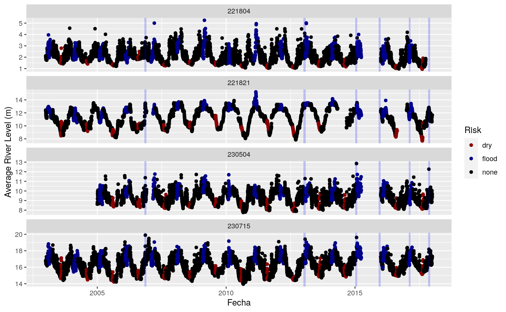
Preliminary observations
There are some interesting patterns to note:
- Two of my upstream stations (Biavo and Huayabamba) appear to have a period of data missing during and after the November 2006 flood. It may be interesting to see how the precipitation data during this period looks. It is understandable that flooding can lead to data gaps.
- All of my stations are missing a big chunk of data in 2015, including the period that corresponds to the December 2015 flood. I am curious to figure out what happened during that time. Was it the flood itself that spurred the re-activation of these stations?
- Many of the flood events reported do not occur during the blue “flood risk” months. I wonder whether my interviewees were misremembering, or if perhaps INDECI has reports on the “out of season” floods, but not the smaller-scale year-after-year types of flash floods.
- Campanilla shows high levels during at least three of the flood “windows”, but no stations shows consistent extremes over all windows.
- There are points at all four stations that seem to correspond to flood-level events, but that do not appear in INDECI reports or my interview results.
Next steps
My next steps will be to try to establish a relationship between regional precipitation and the river level. I think I will have to add some more meteorological stations, based on the juxtaposition of the station to my river gauges. I need to capture precipitation near the gauges, as well as upstream of them. That will be the subject for another post.
This post was compiled on 2020-10-09 18:49:18. Since that time, there may have been changes to the packages that were used in this post. If you can no longer use this code, please notify the author in the comments below.
Packages Used in this post
sessioninfo::package_info(dependencies = "Depends")

#>  package      * version    date       lib source
#>  assertthat     0.2.1      2019-03-21 [1] RSPM (R 4.0.0)
#>  cli            2.0.2      2020-02-28 [1] RSPM (R 4.0.0)
#>  colorspace     1.4-1      2019-03-18 [1] RSPM (R 4.0.0)
#>  crayon         1.3.4      2017-09-16 [1] RSPM (R 4.0.0)
#>  crosstalk      1.1.0.1    2020-03-13 [1] RSPM (R 4.0.0)
#>  curl           4.3        2019-12-02 [1] RSPM (R 4.0.0)
#>  data.table     1.13.0     2020-07-24 [1] RSPM (R 4.0.2)
#>  digest         0.6.25     2020-02-23 [1] RSPM (R 4.0.0)
#>  downlit        0.2.0      2020-09-25 [1] RSPM (R 4.0.2)
#>  dplyr        * 1.0.2      2020-08-18 [1] RSPM (R 4.0.2)
#>  ellipsis       0.3.1      2020-05-15 [1] RSPM (R 4.0.0)
#>  evaluate       0.14       2019-05-28 [1] RSPM (R 4.0.0)
#>  fansi          0.4.1      2020-01-08 [1] RSPM (R 4.0.0)
#>  farver         2.0.3      2020-01-16 [1] RSPM (R 4.0.0)
#>  fs             1.5.0      2020-07-31 [1] RSPM (R 4.0.2)
#>  generics       0.0.2      2018-11-29 [1] RSPM (R 4.0.0)
#>  geosphere      1.5-10     2019-05-26 [1] RSPM (R 4.0.0)
#>  ggplot2      * 3.3.2      2020-06-19 [1] RSPM (R 4.0.1)
#>  glue           1.4.2      2020-08-27 [1] RSPM (R 4.0.2)
#>  gtable         0.3.0      2019-03-25 [1] RSPM (R 4.0.0)
#>  htmltools      0.5.0      2020-06-16 [1] RSPM (R 4.0.1)
#>  htmlwidgets    1.5.1      2019-10-08 [1] RSPM (R 4.0.0)
#>  httr           1.4.2      2020-07-20 [1] RSPM (R 4.0.2)
#>  hugodown       0.0.0.9000 2020-10-08 [1] Github (r-lib/hugodown@18911fc)
#>  jsonlite       1.7.1      2020-09-07 [1] RSPM (R 4.0.2)
#>  knitr          1.30       2020-09-22 [1] RSPM (R 4.0.2)
#>  labeling       0.3        2014-08-23 [1] RSPM (R 4.0.0)
#>  lattice        0.20-41    2020-04-02 [1] RSPM (R 4.0.0)
#>  lazyeval       0.2.2      2019-03-15 [1] RSPM (R 4.0.0)
#>  lifecycle      0.2.0      2020-03-06 [1] RSPM (R 4.0.0)
#>  magrittr       1.5        2014-11-22 [1] RSPM (R 4.0.0)
#>  munsell        0.5.0      2018-06-12 [1] RSPM (R 4.0.0)
#>  pillar         1.4.6      2020-07-10 [1] RSPM (R 4.0.2)
#>  pkgconfig      2.0.3      2019-09-22 [1] RSPM (R 4.0.0)
#>  plotly       * 4.9.2.1    2020-04-04 [1] RSPM (R 4.0.0)
#>  purrr          0.3.4      2020-04-17 [1] RSPM (R 4.0.0)
#>  R6             2.4.1      2019-11-12 [1] RSPM (R 4.0.0)
#>  RColorBrewer   1.1-2      2014-12-07 [1] RSPM (R 4.0.0)
#>  rlang          0.4.7      2020-07-09 [1] RSPM (R 4.0.2)
#>  rmarkdown      2.3        2020-06-18 [1] RSPM (R 4.0.1)
#>  scales         1.1.1      2020-05-11 [1] RSPM (R 4.0.0)
#>  senamhiR     * 0.7.2      2020-10-01 [1] gitlab (ConorIA/senamhiR@b75a2c7)
#>  sessioninfo    1.1.1      2018-11-05 [1] RSPM (R 4.0.0)
#>  sp             1.4-2      2020-05-20 [1] RSPM (R 4.0.0)
#>  stringi        1.5.3      2020-09-09 [1] RSPM (R 4.0.2)
#>  stringr        1.4.0      2019-02-10 [1] RSPM (R 4.0.0)
#>  tibble         3.0.3      2020-07-10 [1] RSPM (R 4.0.2)
#>  tidyr        * 1.1.2      2020-08-27 [1] RSPM (R 4.0.2)
#>  tidyselect     1.1.0      2020-05-11 [1] RSPM (R 4.0.0)
#>  utf8           1.1.4      2018-05-24 [1] RSPM (R 4.0.0)
#>  vctrs          0.3.4      2020-08-29 [1] RSPM (R 4.0.2)
#>  viridisLite    0.3.0      2018-02-01 [1] RSPM (R 4.0.0)
#>  withr          2.3.0      2020-09-22 [1] RSPM (R 4.0.2)
#>  xfun           0.18       2020-09-29 [2] RSPM (R 4.0.2)
#>  yaml           2.2.1      2020-02-01 [1] RSPM (R 4.0.0)
#>  zoo            1.8-8      2020-05-02 [1] RSPM (R 4.0.0)
#>
#> [1] /home/conor/Library
#> [2] /usr/local/lib/R/site-library
#> [3] /usr/local/lib/R/library
Conor I. Anderson, PhD
Alumnus, Climate Lab
Conor is a recent PhD graduate from the Department of Physical and Environmental Sciences at the University of Toronto Scarborough (UTSC).