Revisiting December Temperatures at Toronto
Introduction
In Anderson and Gough ( 2017), Bill Gough and I examined winter temperatures in Toronto, with a special focus on winters 2013/14 and 2014/15. With the recent cold snap, I thought it would be interesting to re-examine the subject. This will all be done in R, with the full code included in this blog post.
First, I will load the libraries that I will use.
library(canadaHCDx)
library(dplyr)
library(ggplot2)
library(readr)
library(tibble)
library(tidyr)
library(zoo)
Now I get the Toronto temperature data:
# Toronto changed station code afer June 2003, so we'll merge it with the new one.
tor <- hcd_daily(5051, 1840:2003)
tmp <- hcd_daily(31688, 2003:2018)
tor <- bind_rows(tor[1:which(tor$Date == "2003-06-30"),], tmp[which(tmp$Date == "2003-07-01"):which(tmp$Date == "2018-01-31"),])
Plots
Let’s first see what the temperature looked like. First, I prepare some “plot data”, extracting December 01 to January 09 (last day of available data so far in 2018).
plot_data <- tor %>% select(Date, MaxTemp, MinTemp, MeanTemp) %>% filter(Date >= "2017-12-01" & Date <= "2018-01-09")
Let’s see what that looks like:
ggplot(data = plot_data) + geom_line(aes(Date, MaxTemp, col = "Tmax")) + geom_line(aes(Date, MinTemp, col = "Tmin")) + geom_hline(aes(yintercept = 0)) + labs(x = "Date", y = "Temperature (°C)", color = "Variable") + ggtitle("Temperature at Toronto (St. George Campus) 2017-12-01 to 2018-01-09") + theme_light()
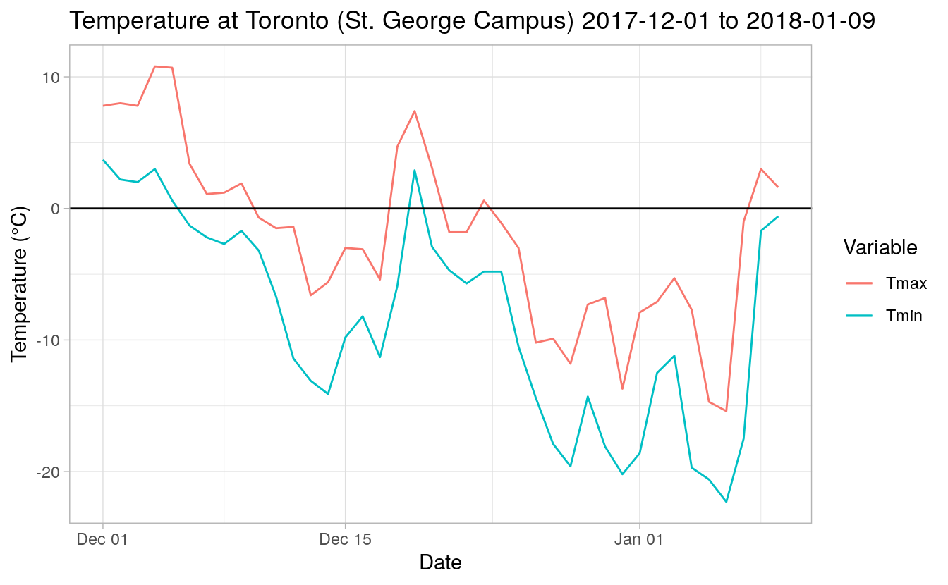
We can see that the beginning of December was fairly mild, with an additional mild period around the 18th to 20th before plummeting in the last days of 2017 and beginning of 2018.
Comparison to daily “normals”
We can’t say for sure that weather is anomalous, unless we compare it to normalized data. Let’s see how December and January look, by plotting the “normal” temperature, i.e. the 30-year average for the same period for each day from 1981–2010.
First, I will generate daily normals by averaging each calendar date over the past 30 years. Note that I am not sure whether this is sloppy methodology, but thought I’d give it a shot.
tor_norm <- tor %>% select(Date, MaxTemp, MinTemp, MeanTemp) %>% filter(format(Date, format = "%Y") >= 1981 & format(Date, format = "%Y") <= 2010)
tor_norm <- tor_norm %>% group_by(Day = format(Date, format = "%m-%d")) %>% summarize_all(mean, na.rm = TRUE) %>% select(-Date)
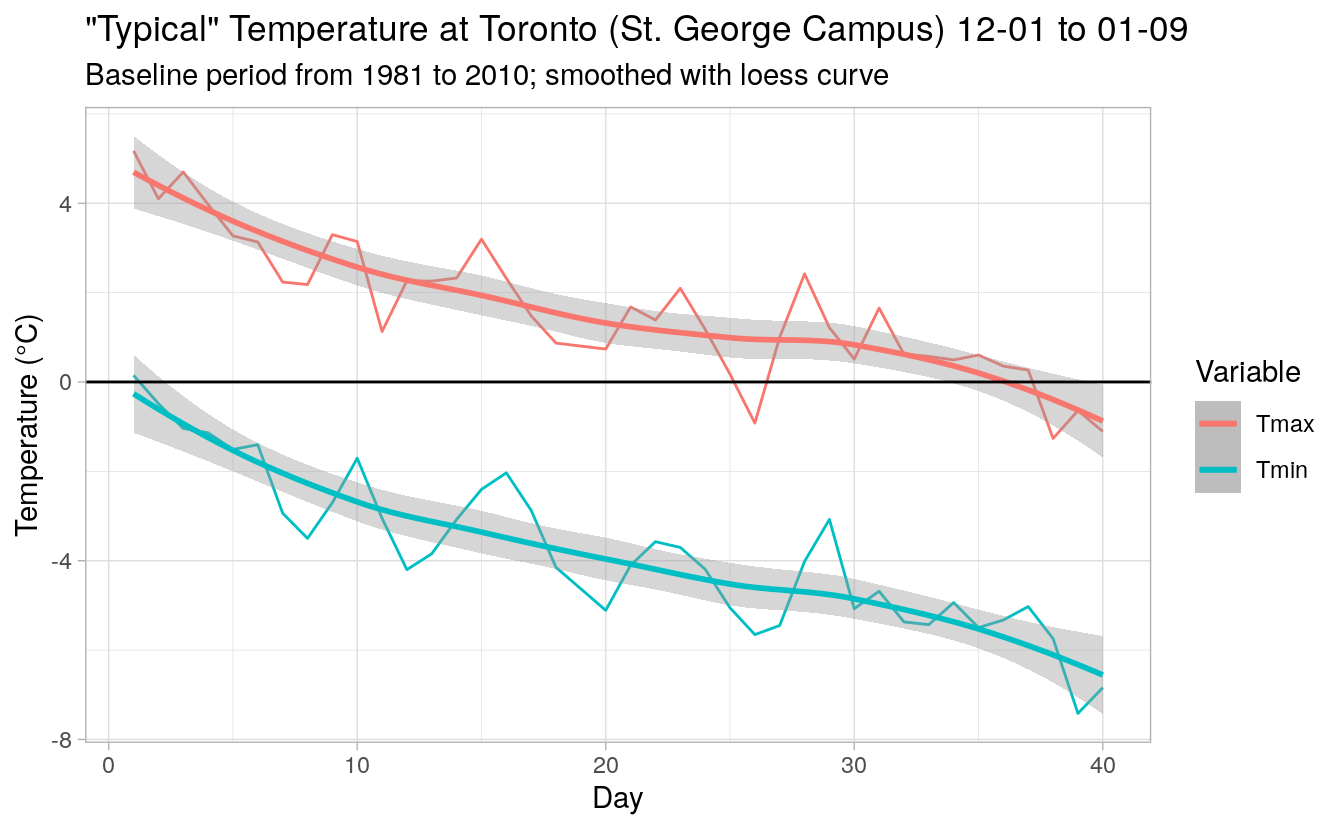
Now that I have the 30-year daily average temperature for each day of the year, I’ll extract just December 1 to January 9. I’ll plot these with a loess curve and use the values from that curve to represent my “typical” temperature.
tor_typical <- bind_rows(tor_norm[tor_norm$Day >= "12-01",], tor_norm[tor_norm$Day <= "01-09",]) %>% add_column(Index = 1:nrow(.)) %>% add_column(MaxSmooth = predict(loess(MaxTemp~Index, .), .$Index), MinSmooth = predict(loess(MinTemp~Index, .), .$Index))

ggplot(data = tor_typical) + geom_line(aes(1:40, MaxTemp, col = "Tmax")) + geom_smooth(aes(1:40, MaxTemp, col = "Tmax")) + geom_line(aes(1:40, MinTemp, col = "Tmin")) + geom_smooth(aes(1:40, MinTemp, col = "Tmin")) + geom_hline(aes(yintercept = 0)) + labs(x = "Day", y = "Temperature (°C)", color = "Variable") + ggtitle("\"Typical\" Temperature at Toronto (St. George Campus) 12-01 to 01-09", subtitle = "Baseline period from 1981 to 2010; smoothed with loess curve") + theme_light()
Now let’s compare our temperature with the “typical”.
plot_data <- plot_data %>% add_column(MaxTempAnom = (.$MaxTemp - tor_typical$MaxSmooth), MinTempAnom = (.$MinTemp - tor_typical$MinSmooth))

ggplot(data = plot_data) + geom_line(aes(Date, MaxTempAnom, col = "Tmax")) + geom_line(aes(Date, MinTempAnom, col = "Tmin")) + geom_hline(aes(yintercept = 0))+ labs(x = "Day", y = "Temperature Anomaly (°C)", color = "Variable") + ggtitle("Temperature Anomaly at Toronto 2017-12-01 to 2018-01-09", subtitle = "Relative to smoothed 1981-2010 baseline") + theme_light()
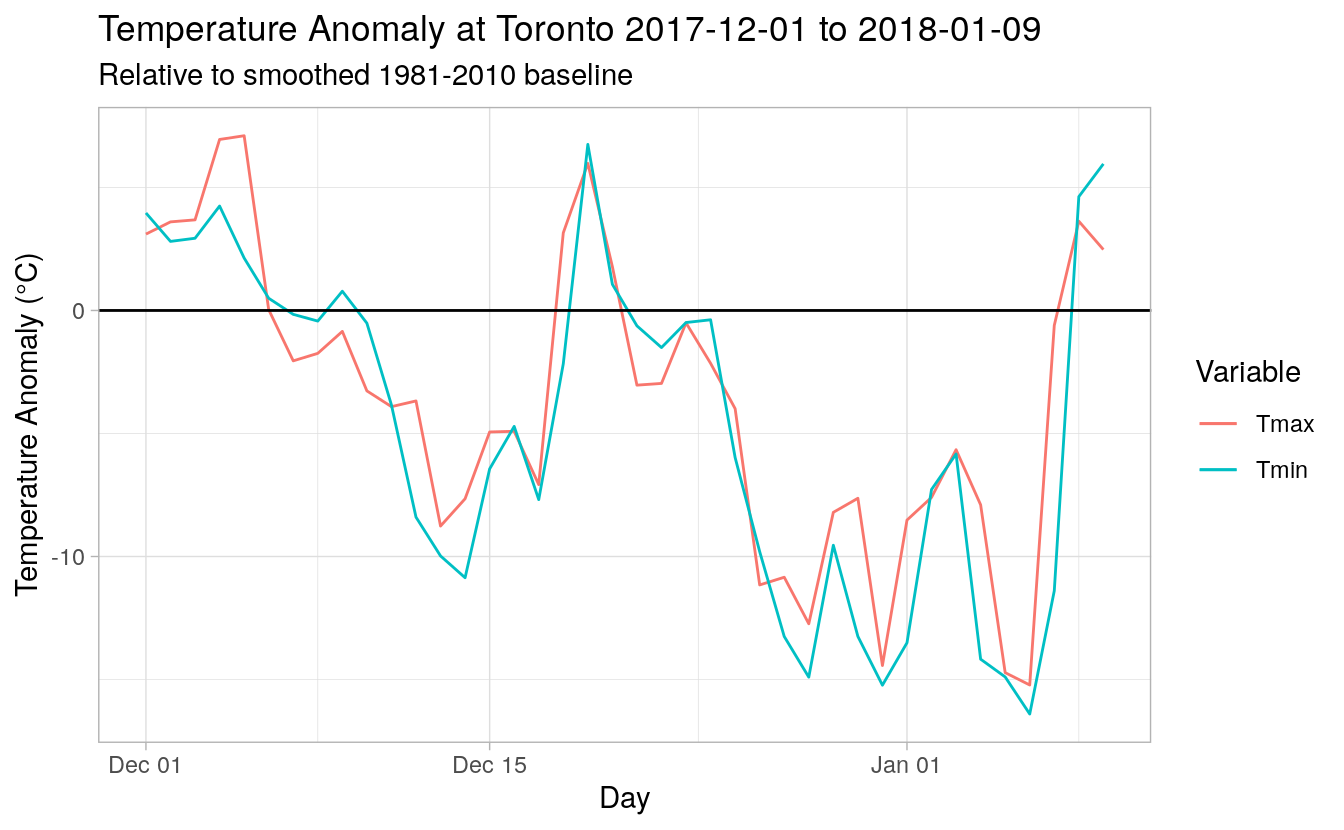
Indeed, temperatures were cold, getting to be as much as 16 °C colder than the smoothed average daily temperature from 1981–2010.
How does December rank?
Now let’s prepare some December-only data series at the daily and monthly timescales.
tor_dec <- tor %>% select(Date, MaxTemp, MinTemp, MeanTemp) %>% filter(format(Date, format = "%m") == 12)
tor_dec_mon <- tor_dec %>% group_by(Yearmon = format(Date, format = "%Y-%m")) %>% summarize_all(mean, na.rm = TRUE)
Note, I have become largely familiar with the Toronto data series, and I know that missing data is not an issue in this time series. Generally, one would need to do a quick check of the data, such as:
quick_audit(tor_dec, c("MaxTemp", "MinTemp", "MeanTemp"), by = "month")

#> # A tibble: 178 x 6
#>    Year  Month `Year-month` `MaxTemp pct NA` `MinTemp pct NA` `MeanTemp pct NA`
#>    <chr> <chr> <yearmon>               <dbl>            <dbl>             <dbl>
#>  1 1840  12    Dec 1840                    0                0                 0
#>  2 1841  12    Dec 1841                    0                0                 0
#>  3 1842  12    Dec 1842                    0                0                 0
#>  4 1843  12    Dec 1843                    0                0                 0
#>  5 1844  12    Dec 1844                    0                0                 0
#>  6 1845  12    Dec 1845                    0                0                 0
#>  7 1846  12    Dec 1846                    0                0                 0
#>  8 1847  12    Dec 1847                    0                0                 0
#>  9 1848  12    Dec 1848                    0                0                 0
#> 10 1849  12    Dec 1849                    0                0                 0
#> # … with 168 more rows
OK, let’s look at some monthly ranks!
tor_dec_mon <- tor_dec_mon %>% add_column(MaxTempRank = min_rank(.$MaxTemp), MinTempRank = min_rank(.$MinTemp), MeanTempRank = min_rank(.$MeanTemp))

tail(tor_dec_mon)

#> # A tibble: 6 x 8
#>   Yearmon Date       MaxTemp MinTemp MeanTemp MaxTempRank MinTempRank
#>   <chr>   <date>       <dbl>   <dbl>    <dbl>       <int>       <int>
#> 1 2012-12 2012-12-16   4.76   -0.827    1.94          171         173
#> 2 2013-12 2013-12-16  -0.567  -5.60    -3.24           45          81
#> 3 2014-12 2014-12-16   3.25   -1.57     0.857         148         163
#> 4 2015-12 2015-12-16   7.57    2.52     5.06          178         178
#> 5 2016-12 2016-12-16   2.23   -2.97    -0.387         125         139
#> 6 2017-12 2017-12-16  -0.845  -6.94    -3.91           36          46
#> # … with 1 more variable: MeanTempRank <int>
Toronto’s temperature in the month of December 2017 was ranked 36 for $T_{max}$ (-0.845 °C with a return interval (RI) of 4.97) , 46 for $T_{min}$ (-6.94 °C with RI of 3.89), and 40 for $T_{mean}$ (-3.91 °C with RI of 4.47). All three variables are ranked out of 178 total Decembers in the set.
The last time that we saw a December this cold was in 2000-12. The temperature that year was:
- $T_{max}$: -2.11 °C, rank 12, with RI of 14.9
- $T_{min}$: -7.73 °C, rank 34, with RI of 5.26
- $T_{mean}$: -4.94 °C, rank 24, with RI of 7.46
The second-last December that was as cold or colder than December 2017 was 1989-12. That year the temperature reached:
- $T_{max}$: -4.63 °C, rank 1, with RI of 179
- $T_{min}$: -10.9 °C, rank 3, with RI of 59.7
- $T_{mean}$: -7.79 °C, rank 3, with RI of 59.7
Air Mass Analysis
One of the things that we looked at in our 2017 paper was the position of the jet stream. During December 2017, we know that the jet stream was to the south of Toronto during the cold snap. Let’s look at this, using data from Sheridan’s Spatial Synoptic Classification (SSC) (Sheridan 2002).
First, I’ll get the data and bin it into four bins, as per Anderson and Gough ( 2017):
- ‘cool’: SSC codes 2 (dry polar) and 5 (moist polar)
- ‘moderate’: SSC codes 1 (dry moderate) and 4 (moist moderate)
- ‘warm’: SSC codes 3 (dry tropical), 6 (moist tropical), 66 (moist tropical plus), and 67 (moist tropical double plus)
- ‘transition’: SCC code 7 (transition)
f <- tempfile()
download.file("http://sheridan.geog.kent.edu/ssc/files/YYZ.dbdmt", f, quiet = TRUE)
air <- read_table(f, col_names = c("Station", "Date", "Air"), col_types = cols(col_character(), col_date(format = "%Y%m%d"), col_factor(levels = c(1, 2, 3, 4, 5, 6, 7, 66, 67)))) # Note, I am ignoring code 8 because that is the SSC2 "NA" value, which is turned to NA by ignoring.
levels(air$Air) <- list(cool = c(2, 5), mod = c(1, 4), warm = c(3, 6, 66, 67), trans = "7")
Now I will rearrange so that I get the proportions of each.
# Some hints from https://stackoverflow.com/questions/25811756/summarizing-counts-of-a-factor-with-dplyr

air_dec <- air %>% filter(format(Date, format = "%m") == 12)
air_tally <- air_dec %>% select(-Station) %>% group_by(Yearmon = as.yearmon(Date), Air) %>% tally %>% spread(Air, n, fill = 0)
air_tally <- air_tally %>% filter(`<NA>` < 31) # Remove empty year-months
air_prop <- as_tibble(prop.table(as.matrix(air_tally[,2:ncol(air_tally)]), 1))
names(air_prop) <- paste(names(air_prop), "prop", sep = "_")
air_prop <- bind_cols(air_tally, air_prop)
The last few Decembers, for instance:
tail(air_prop) %>% select(-2:-6)

#> # A tibble: 6 x 6
#> # Groups:   Yearmon [6]
#>   Yearmon   cool_prop mod_prop warm_prop trans_prop `<NA>_prop`
#>   <yearmon>     <dbl>    <dbl>     <dbl>      <dbl>       <dbl>
#> 1 Dec 2012      0.323    0.581    0.0323     0.0645      0
#> 2 Dec 2013      0.613    0.290    0          0.0968      0
#> 3 Dec 2014      0.484    0.355    0.0645     0.0968      0
#> 4 Dec 2015      0.161    0.613    0.129      0.0968      0
#> 5 Dec 2016      0.548    0.323    0          0.0968      0.0323
#> 6 Dec 2017      0.548    0.323    0          0.129       0
So, was it just the origin of the air that made December so cold? Not exactly. on average 57.1% of daily December air masses are of polar origin. We had 54.8% air of polar origin in December 2017.
Let’s take a look at the continuity of the polar air. Here I will look for the longest continuous series of ‘cool’ or ‘trans’ air for each December, omitting any missing values. Therefore, for this analysis, a cold snap is the longest period of two or more consecutive days of polar or transitional air during each December.
# Took some code from https://stackoverflow.com/questions/41254014/consecutive-count-by-groups

fx <- function(x) {
  x <- na.omit(x)
  if (length(x) > 0) {
    with(rle(x == "cool" | x == "trans"), max(lengths[values]))
  } else {
    NA
  }
}


air_consec <- air_dec %>%
   group_by(Year = format(Date, format = "%Y")) %>%
      summarise(ConsecutivePolar = fx(Air))

#> `summarise()` ungrouping output (override with `.groups` argument)


tail(air_consec)

#> # A tibble: 6 x 2
#>   Year  ConsecutivePolar
#>   <chr>            <int>
#> 1 2012                 5
#> 2 2013                13
#> 3 2014                 5
#> 4 2015                 2
#> 5 2016                12
#> 6 2017                11
So, was it the length of the cold snap that made December so cold?: So far, no! The cold snap (up to December 31) was only 11 days long. Since 1950, 25 Decembers showed cold snaps that were longer than the 2017 one and 39 Decembers showed maximum cold snaps that were as long or shorter. It looks like the length of our snap is pretty near the middle.1 This is interesting to compare to the Decembers with the longest cold snaps (which also happen to include the most recent colder Decembers:
- Year 1989, length of cold snap: 30
- Year 1950, length of cold snap: 28
- Year 2000, length of cold snap: 27
December 2017 was ranked highly in terms of how cold it got, even with a relatively short period of arctic air in the month.
Conclusions
From what I can tell, it wasn’t a case of the origin or length of the December cold snap that was anomalous.2 Instead, we just got some very, very cold temperatures that were between 6 and 16 °C colder than the temperatures that we would typically expect for the period from, December 21 to January 9, with the strongest anomalies from December 26 to around January 6th. Note, however, that other scientists have reached the opposite conclusion (that the length was more remarkable than the temperature). Another group directly contradicts that previous article. The debate rages on!
This post was compiled on 2020-10-09 11:29:27. Since that time, there may have been changes to the packages that were used in this post. If you can no longer use this code, please notify the author in the comments below.
Packages Used in this post
sessioninfo::package_info(dependencies = "Depends")

#>  package     * version    date       lib source
#>  assertthat    0.2.1      2019-03-21 [1] RSPM (R 4.0.0)
#>  canadaHCD   * 0.0-2      2020-10-01 [1] Github (ConorIA/canadaHCD@e2f4d2b)
#>  canadaHCDx  * 0.0.8      2020-10-01 [1] gitlab (ConorIA/canadaHCDx@0f99419)
#>  cli           2.0.2      2020-02-28 [1] RSPM (R 4.0.0)
#>  colorspace    1.4-1      2019-03-18 [1] RSPM (R 4.0.0)
#>  crayon        1.3.4      2017-09-16 [1] RSPM (R 4.0.0)
#>  curl          4.3        2019-12-02 [1] RSPM (R 4.0.0)
#>  digest        0.6.25     2020-02-23 [1] RSPM (R 4.0.0)
#>  downlit       0.2.0      2020-09-25 [1] RSPM (R 4.0.2)
#>  dplyr       * 1.0.2      2020-08-18 [1] RSPM (R 4.0.2)
#>  ellipsis      0.3.1      2020-05-15 [1] RSPM (R 4.0.0)
#>  evaluate      0.14       2019-05-28 [1] RSPM (R 4.0.0)
#>  fansi         0.4.1      2020-01-08 [1] RSPM (R 4.0.0)
#>  farver        2.0.3      2020-01-16 [1] RSPM (R 4.0.0)
#>  fs            1.5.0      2020-07-31 [1] RSPM (R 4.0.2)
#>  generics      0.0.2      2018-11-29 [1] RSPM (R 4.0.0)
#>  geosphere     1.5-10     2019-05-26 [1] RSPM (R 4.0.0)
#>  ggplot2     * 3.3.2      2020-06-19 [1] RSPM (R 4.0.1)
#>  glue          1.4.2      2020-08-27 [1] RSPM (R 4.0.2)
#>  gtable        0.3.0      2019-03-25 [1] RSPM (R 4.0.0)
#>  hms           0.5.3      2020-01-08 [1] RSPM (R 4.0.0)
#>  htmltools     0.5.0      2020-06-16 [1] RSPM (R 4.0.1)
#>  hugodown      0.0.0.9000 2020-10-08 [1] Github (r-lib/hugodown@18911fc)
#>  knitr         1.30       2020-09-22 [1] RSPM (R 4.0.2)
#>  labeling      0.3        2014-08-23 [1] RSPM (R 4.0.0)
#>  lattice       0.20-41    2020-04-02 [1] RSPM (R 4.0.0)
#>  lifecycle     0.2.0      2020-03-06 [1] RSPM (R 4.0.0)
#>  magrittr      1.5        2014-11-22 [1] RSPM (R 4.0.0)
#>  Matrix        1.2-18     2019-11-27 [1] RSPM (R 4.0.0)
#>  mgcv          1.8-33     2020-08-27 [1] RSPM (R 4.0.2)
#>  munsell       0.5.0      2018-06-12 [1] RSPM (R 4.0.0)
#>  nlme          3.1-149    2020-08-23 [1] RSPM (R 4.0.2)
#>  pillar        1.4.6      2020-07-10 [1] RSPM (R 4.0.2)
#>  pkgconfig     2.0.3      2019-09-22 [1] RSPM (R 4.0.0)
#>  purrr         0.3.4      2020-04-17 [1] RSPM (R 4.0.0)
#>  R6            2.4.1      2019-11-12 [1] RSPM (R 4.0.0)
#>  rappdirs      0.3.1      2016-03-28 [1] RSPM (R 4.0.0)
#>  Rcpp          1.0.5      2020-07-06 [1] RSPM (R 4.0.2)
#>  readr       * 1.3.1      2018-12-21 [1] RSPM (R 4.0.2)
#>  rlang         0.4.7      2020-07-09 [1] RSPM (R 4.0.2)
#>  rmarkdown     2.3        2020-06-18 [1] RSPM (R 4.0.1)
#>  scales        1.1.1      2020-05-11 [1] RSPM (R 4.0.0)
#>  sessioninfo   1.1.1      2018-11-05 [1] RSPM (R 4.0.0)
#>  sp            1.4-2      2020-05-20 [1] RSPM (R 4.0.0)
#>  storr         1.2.1      2018-10-18 [1] RSPM (R 4.0.0)
#>  stringi       1.5.3      2020-09-09 [1] RSPM (R 4.0.2)
#>  stringr       1.4.0      2019-02-10 [1] RSPM (R 4.0.0)
#>  tibble      * 3.0.3      2020-07-10 [1] RSPM (R 4.0.2)
#>  tidyr       * 1.1.2      2020-08-27 [1] RSPM (R 4.0.2)
#>  tidyselect    1.1.0      2020-05-11 [1] RSPM (R 4.0.0)
#>  utf8          1.1.4      2018-05-24 [1] RSPM (R 4.0.0)
#>  vctrs         0.3.4      2020-08-29 [1] RSPM (R 4.0.2)
#>  withr         2.3.0      2020-09-22 [1] RSPM (R 4.0.2)
#>  xfun          0.18       2020-09-29 [2] RSPM (R 4.0.2)
#>  yaml          2.2.1      2020-02-01 [1] RSPM (R 4.0.0)
#>  zoo         * 1.8-8      2020-05-02 [1] RSPM (R 4.0.0)
#>
#> [1] /home/conor/Library
#> [2] /usr/local/lib/R/site-library
#> [3] /usr/local/lib/R/library
References
Anderson, Conor I., and William A. Gough. 2017. “Evolution of Winter Temperature in Toronto, Ontario, Canada: A Case Study of Winters 2013/14 and 2014/15.” Journal of Climate 30 (14): 5361–76. https://doi.org/10.1175/JCLI-D-16-0562.1.
Sheridan, Scott C. 2002. “The Redevelopment of a Weather-Type Classification Scheme for North America.” International Journal of Climatology 22 (1): 51–68. https://doi.org/10.1002/joc.709.
-
Note, this only considers December (no SSC data for January yet), so this is definitely subject to change, since the cold snap was limited to the end of December and start of January. At this point, one conclusion to draw from this is that long cold snaps typically start earlier in December than the 2017/18 one. ↩︎
-
Again, I was just looking at December air masses here, this is likely to change when we consider the January days; there are also other ways to think about the length of the cold snap e.g. number of consecutive days that are more than $x$ degrees below the baseline, that I have not considered here. ↩︎
Conor I. Anderson, PhD
Alumnus, Climate Lab
Conor is a recent PhD graduate from the Department of Physical and Environmental Sciences at the University of Toronto Scarborough (UTSC).