Twitter abuse of Canada's Environment Minister, Catherine McKenna
On September 8 it was reported that Catherine McKenna now requires IRL security after enduring years of escalating abuse on Twitter. I, of course, was perturbed by the vitriol that I had seen directed at the minister, but I had largely dismissed it as part and parcel of Twitter. Twitter is a strange microcosm of some of the worst elements of politics—a sort of strange other world where earnest human tweeters, bot networks, and other shadowy figures all share “thoughts”; sometimes it is hard to tell who is sincere, who is a troll, and who is nothing more than a couple of lines of code on a server somewhere. As a climate scientist, I am always interested to see how social media platforms amplify climate change denial, or push regressive climate (in)action policy positions. I thought that Catherine McKenna’s Twitter world would be a great case study, and I wanted to see if there was any specific milestone that marked a significant shift in the tone of Tweets that are directed at her.
Usually when I create a write-up like this, I share the full methodology, but today I am going to omit the specific lines of code that were used to obtain the Tweet data that I analyzed. Twitter has an official API, which allows free access to the last 9 days of history. Paid access will allow access to the full Twitter archive. There are myriad tutorials online to help use the API. An alternative option is to script interactions between a web browser and Twitter. Programming a browser to visit Twitter automatically is probably ethical, but very likely in contravention of Twitter ToS, so be cautious if you want to undertake an analysis of that sort.
For this analysis, I will be using an object called tweets that contains five columns: the timestamp the tweet was sent (timstamp); the Status ID of the top tweet in the thread (reply_to), the Status ID of each individual Tweet (twid), the username of the tweeter (user), and the Tweet text (tweet).
Let’s start by loading the libraries that we will use through this analysis.
library(dplyr)
library(ggplot2)
library(readr)
library(stringr)
library(tibble)
library(tidyr)
library(tidytext)
library(wordcloud2)
library(zoo)
Now I will clean up some duplicate entries in my data and filter to a fixed range of dates.
tweets %>%
  distinct(twid, .keep_all = TRUE) %>%
  filter(as.Date(timestamp) >= "2015-11-04" &
         as.Date(timestamp) <= "2019-09-08")-> tweets
I will only look at Tweets between November 4, 2015 (the day that McKenna assumed office as Environment Minister), and September 8, 2019 (the day it was reported that she required security). The dataset I used contained 247226 Tweets in 12989 threads. Catherine McKenna wrote 13308 of the Tweets, and was, of course, the first tweeter in each thread. I should note that this analysis only includes replies, and does not include unthreaded Tweets direct to @cathmckenna or any direct messages she may receive.
Let’s first look at the raw breakdown of Tweet volume by day.
tweets %>%
  filter(user == "cathmckenna") %>%
  group_by(Day = as.Date(timestamp)) %>%
  count() %>%
  filter(Day >= "2015-11-04" & Day <= "2019-09-08") %>%
  ggplot(aes(x = Day, y = n)) +
  geom_line(color = "#34495E") +
  ggtitle("Tweets authored by @cathmckenna, by day",
          subtitle = "Nov. 4, 2015 to Sep. 8, 2019")
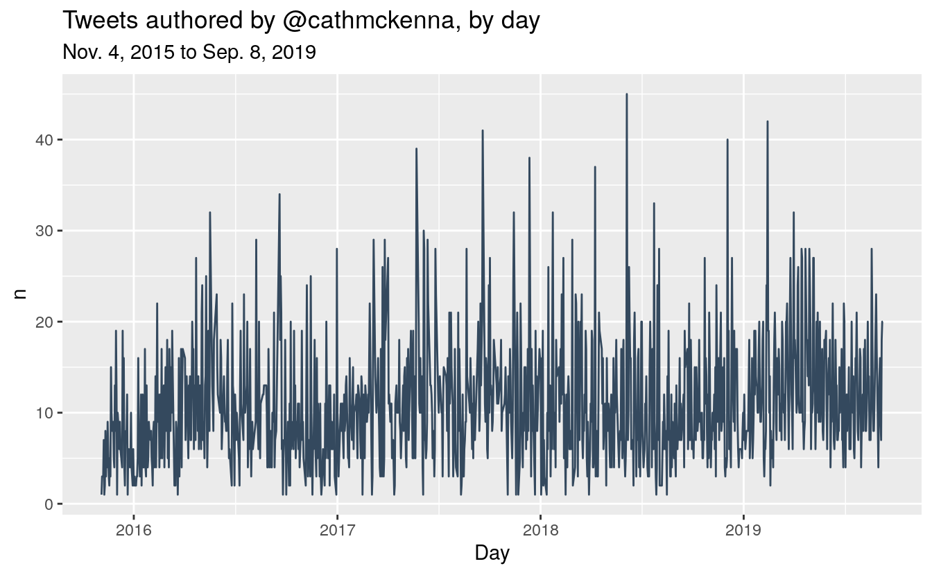
McKenna is a heavy Twitter user, and we can see some spikes on which she sent a very high volume of Tweets. Her biggest day was on June 5, 2018, World Environment Day, followed by February 13, 2019, when McKenna released a series of Tweets defending the federal carbon tax (to coincide with Saskatchewan’s court challenge to the tax’s constitutionality). Her third biggest day was from the 72nd UN General Assembly on September 19, 2019.
Now let’s see the reply volume by day.
tweets %>%
  filter(user != "cathmckenna") %>%
  group_by(Day = as.Date(timestamp)) %>%
  count() %>%
  filter(Day >= "2015-11-04" & Day <= "2019-09-08") %>%
  ggplot(aes(x = Day, y = n)) +
  geom_vline(xintercept = as.Date("2019-04-01"), colour = "red", linetype = "dashed") +
  geom_line(color = "#34495E") +
  ggtitle("@cathmckenna reply volume, by day",
          subtitle = "Nov. 4, 2015 to Sep. 8, 2019")
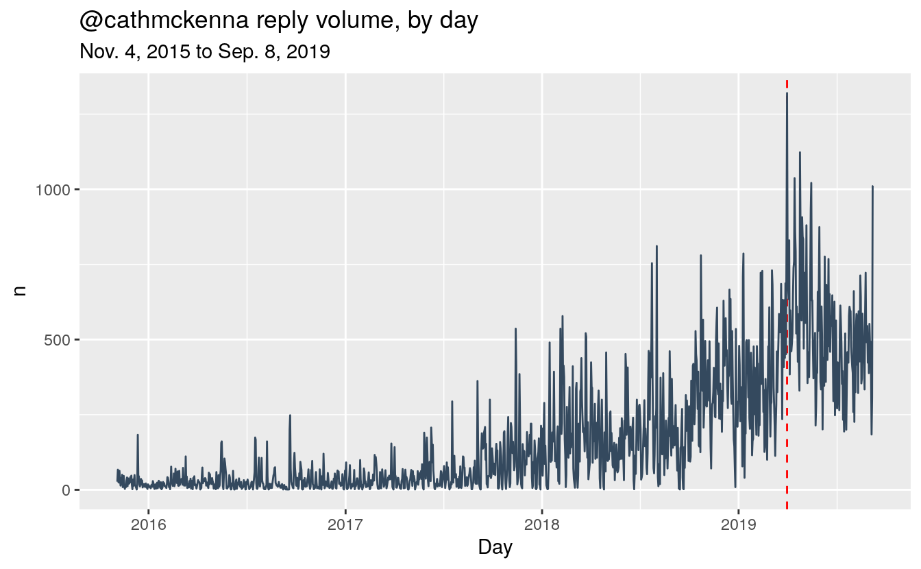
By far the highest volume of Tweets directed to McKenna was sent on April 1, 2019 (marked with a dash red line). April 1 was the day the federal carbon tax took effect in Ontario, Saskatchewan, Manitoba and New Brunswick. Other high-volume days were April 25, April 15, May 16, and September 8. I didn’t find any standout issue on April 15, 25 or May 16. September 8 seems to have been a mix of McKenna’s defenders (“can’t believe you have to go through this”) and abusers (“playing the victim card”) reacting to her announcement that she required a security detail. Later in this notebook, I will show the Tweets from McKenna that garnered the most replies.
Let’s first take a look a who the most prolific tweeters are on Cath McKenna’s statuses.
tweets %>%
  group_by(user) %>%
  filter(user != "cathmckenna") %>%
  count() -> tweet_volume
tweet_volume %>% arrange(desc(n))

#> # A tibble: 28,453 x 2
#> # Groups:   user [28,453]
#>    user                n
#>    <chr>           <int>
#>  1 kgaider          2364
#>  2 FriendsOScience  1091
#>  3 erwingerrits      927
#>  4 bo_canut          867
#>  5 Darrylrides       826
#>  6 isma_fan          779
#>  7 FraserMacLeod5    772
#>  8 NecktopP          671
#>  9 OldWood007        650
#> 10 stan15537715      632
#> # … with 28,443 more rows
Kathy Gaider (@kgaider) is the most prolific tweeter by far. At the time of writing, Gaider’s account was suspended, but the snippet of her bio from a DuckDuckGo search reveals a strong anti-Liberal bent and an assertion of holding “three real science degrees”. So take that for what its worth. Twitter users informed me that Kathy was (or claimed to be) an ex-Environment Canada employee who unleashed a series of ad-hominen attacks on Trudeau and McKenna. Gaider’s supporters claim that her account was suspended after she revealed data manipulation by Environment Canada. I reached out to a contact at ECCC to see if he had heard about this, but he was on vacation when I got in touch. At any rate, I have found no evidence (nor do I believe) that Environment Canada engaged in any manipulation of data. Data is often corrected to account for measuring errors or other systematic quality control issues. Snopes even has a write up on the topic.
Number two on the list are the mind-numbingly oxymoronic climate change denial crusaders behind the “Friends of Science” moniker. FoS are known climate denial trolls and are wilfully ignorant of modern climate science. The members of the group remain anonymous, but they have been linked to fossil fuel interests.
User number 3, @, is another anti-Liberal Twitter activist, judging from his profile photo at the time of writing: a Liberal “L” logo embedded in the word “Liars”. I don’t want to explore all of the above users just now, but I am sure that many more on the list may similar anti-Liberal biases. I think it is a safe assumption to say that Catherine McKenna isn’t inundated with loving Tweets.
tweet_volume %>%
  arrange(desc(n)) %>%
  select(user) %>%
  head(5) %>%
  unlist() -> top_tweeters

tweets %>%
  filter(user %in% top_tweeters) %>%
  group_by(user, month = as.yearmon(timestamp)) %>%
  count() %>%
  ggplot(aes(x = month, y = n, fill = user)) +
  geom_col() +
  scale_x_continuous() + ggtitle("Top five most prolific tweeters in replies directed to @cathmckenna")
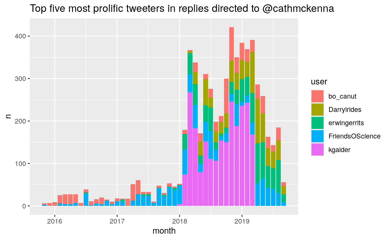
We can see a pattern of concentrated effort from 2018 to present. It seems Gaider was either suspended just before April of this year. This is an interesting point, because that means that Gaider didn’t contribute to the explosion of Tweets on April 1, 2019, unless it was under another account name.
Tokens
What can we learn about the content of these Tweets? Let’s perform some quick text mining. I’ll start by tokenizing the Tweets. First, I will remove “rt”, usernames, punctuation, URLs, and tabs, and then trim whitespace. Finally, I’ll remove common stop words in both English and French (McKenna tweets in both languages).
data(stop_words)
# Clean up tweet text
tweets$tweet %>% tolower %>%
  str_remove_all(pattern = "^rt|@[^\\s]+|https?[^\\s]+|pic\\.twitter\\.com[^\\s]+|[[:punct:]]") %>%
  str_trim -> tweets$tweet

# unnest tokens and remove stop words
tweets %>%
  unnest_tokens(word, tweet) %>%
  anti_join(stop_words, by = "word") %>%
  anti_join(
    tibble(
      word = jsonlite::fromJSON(
        "https://raw.githubusercontent.com/stopwords-iso/stopwords-iso/master/stopwords-iso.json")$fr),
    by = "word") -> tokens
Let’s see a wordcloud of McKenna’s Tweets.
tokens %>%
  filter(user == "cathmckenna") %>%
  count(word, sort = TRUE) %>%
  wordcloud2()
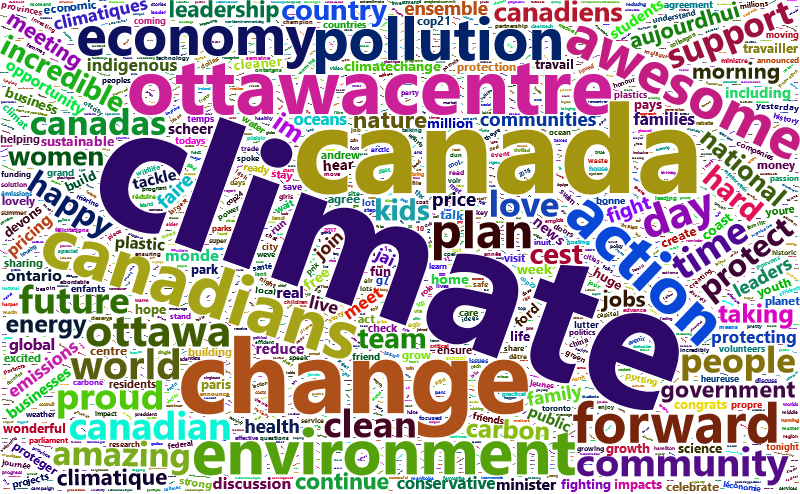
The content here makes sense for a person in her position. We can see words that appeal to her riding, her portfolio, and to Canadians in general.
How about the replies?
tokens %>%
  filter(user != "cathmckenna") %>%
  count(word, sort = TRUE) %>%
  wordcloud2()
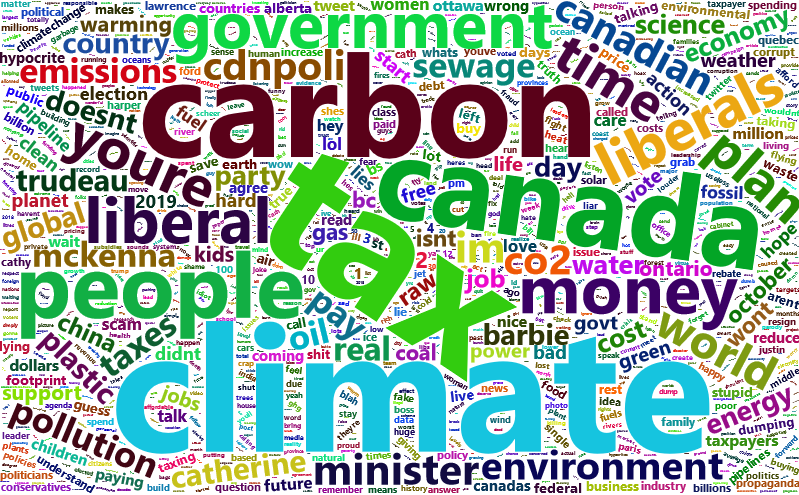
The content of the replies contains words that focus on the carbon tax, and terms that seem be personal and party references. A number of insults and slurs have a fairly high precedence.
Let’s look at the “sentiment”–whether they are positive or negative–of all of the words in the replies. I’ll use a sentiment lexicon developed by Nielsen ( 2011). This lexicon rates words on a scale of -5 to 5, scored for valence. Not all words will be captured by this lexicon, so this analysis won’t capture everything, but will rather look for key words in Tweets. Sentiment analysis is not a perfect science, since it scores words independent of their context, but it is a good way to get a sense of the general tone of the corpus of Tweets.
You can access the AFINN 111 word list in R using
get_sentiments("afinn") from the tidytext package, but that can’t be done non-interactively, so won’t work on this blog. I will use JSON to grab AFINN 165, which contains 905 more words than 111.
afinn <- jsonlite::fromJSON("https://raw.githubusercontent.com/words/afinn-165/master/index.json")
afinn <- tibble(word = names(afinn), value = unlist(afinn))
token_sentiment <- tokens %>% full_join(afinn, by = "word")
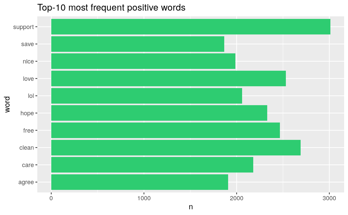
These are the top-10 positive words in the comments:
token_sentiment %>% filter(value > 0) %>% count(word, sort = TRUE) %>% head(10) %>%
  ggplot(aes(word, n)) + geom_col(fill = "#2ECC71") + coord_flip() +
  ggtitle("Top-10 most frequent positive words")
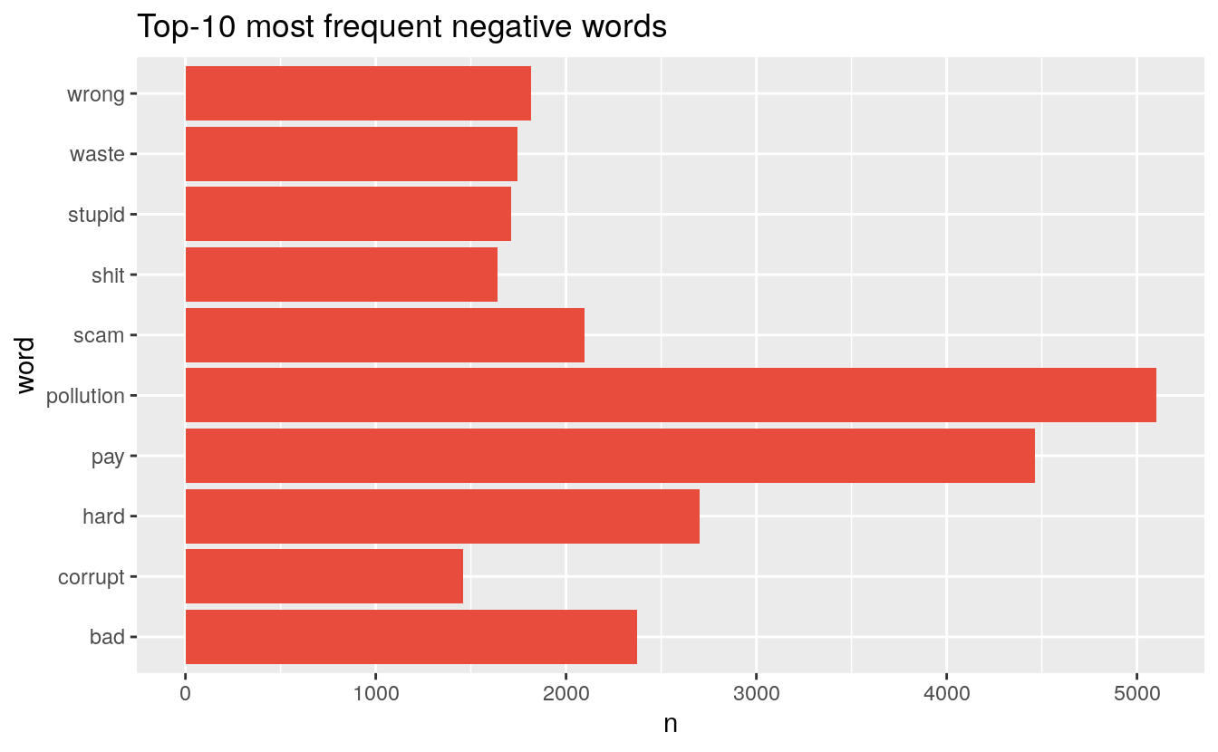
These are the top-10 negative words in the comments:
token_sentiment %>% filter(value < 0) %>% count(word, sort = TRUE) %>% head(10) %>%
  ggplot(aes(word, n)) + geom_col(fill = "#E74C3C") + coord_flip() +
  ggtitle("Top-10 most frequent negative words")
Tweet sentiment
Later we can look at word frequencies, but let’s go back to using Tweets as a unit. We can get a rough idea of the sentiment of a Tweet by averaging the sentiment of the constituent words in the Tweet.
token_sentiment %>%
  group_by_at(vars(-word, -value)) %>%
  summarize(sentiment = mean(value, na.rm = TRUE)) %>%
  right_join(tweets, by = c("timestamp", "reply_to", "twid", "user")) %>%
  ungroup() -> tweet_sentiment

#> `summarise()` regrouping output by 'timestamp', 'reply_to', 'twid' (override with `.groups` argument)
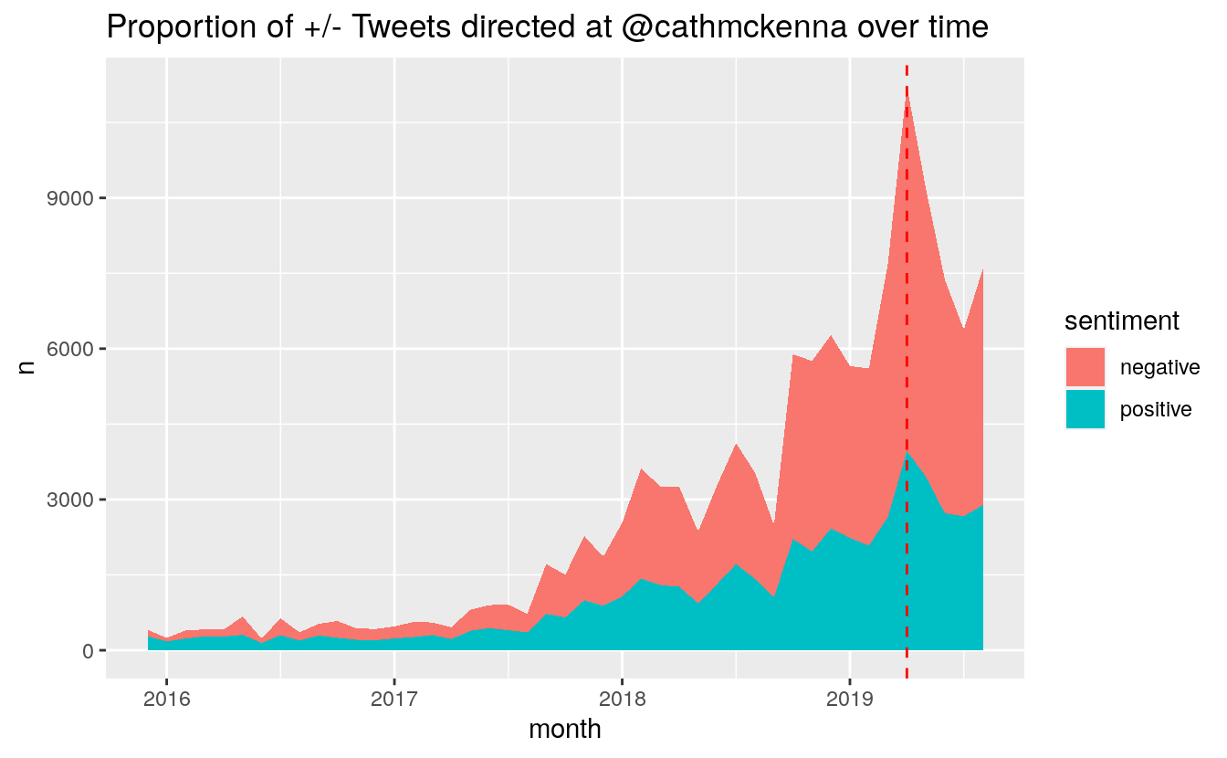
Let’s see how the average sentiment of Tweets in the Catherine McKenna orbit have changed over time. Unsurprisingly, Cath McKenna is the most positive voice on her own twitter, so let’s look at just the replies to her Tweets.
tweet_sentiment %>%
  filter(user != "cathmckenna" & !is.na(sentiment)) %>%
  mutate(month = as.yearmon(timestamp)) %>%
  select(month, user, sentiment) %>%
  group_by(month) %>%
  summarize(positive = sum(sentiment > 0), negative = sum(sentiment <0), sentiment = mean(sentiment)) -> monthly_sentiment

#> `summarise()` ungrouping output (override with `.groups` argument)
We can look at the count value of positive and negative Tweets:
monthly_sentiment %>%
  filter(month > "2015-11" & month < "2019-09") %>%
  select(-sentiment) %>%
  pivot_longer(cols = 2:3, names_to = "sentiment", values_to = "n") %>%
  ggplot(aes(month, n, fill = sentiment)) + geom_area() +
  scale_x_continuous() +
  geom_vline(xintercept = as.yearmon("2019-04"), colour = "red", linetype = "dashed") +
  ggtitle("Proportion of +/- Tweets directed at @cathmckenna over time")
Changes in the proportion of positive and negative Tweets:
monthly_sentiment %>%
  filter(month > "2015-11" & month < "2019-09") %>%
  mutate(total = positive + negative,
         positive = positive / total,
         negative = negative / total) %>%
  select(-sentiment, -total) %>%
  pivot_longer(cols = 2:3, names_to = "sentiment", values_to = "n") %>%
  ggplot(aes(month, n, colour = sentiment)) + geom_line() +
  scale_x_continuous() +
  ggtitle("Proportion of positive and negative Tweets directed at @cathmckenna over time")
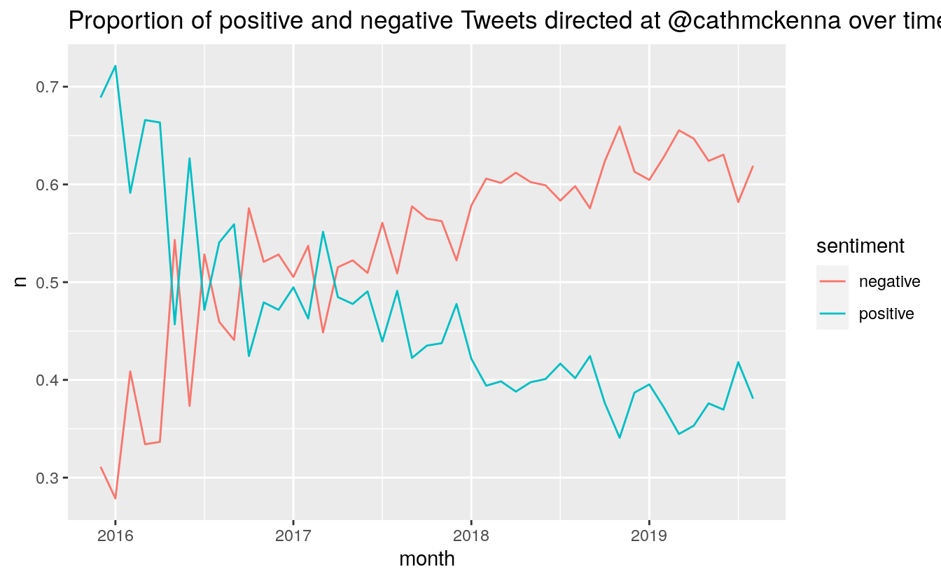
It is interesting to note that March 2019 was actually the month with the lowest average sentiment. November 2018, the month after the IPCC SR15 report, and the month before COP24, ranked second. April 2019 was the third most negative month.
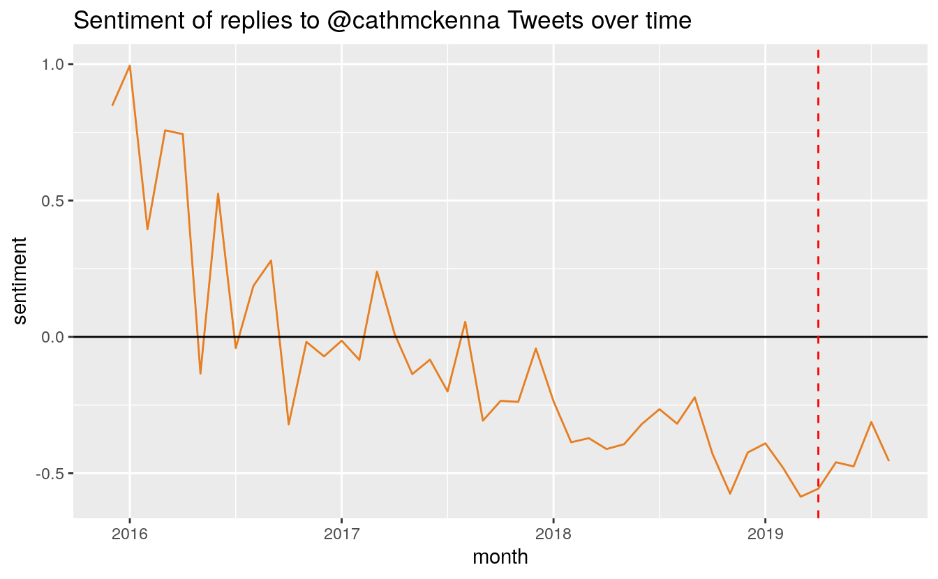
We can also look at changes in the average sentiment of all replies in a month:
monthly_sentiment %>%
  filter(month > "2015-11" & month < "2019-09") %>%
  ggplot(aes(month, sentiment)) + geom_line(show.legend = FALSE, color = "#E67E22") +
  geom_hline(aes(yintercept = 0)) +
  scale_x_continuous() +
  geom_vline(xintercept = as.yearmon("2019-04"), colour = "red", linetype = "dashed") +
  ggtitle("Sentiment of replies to @cathmckenna Tweets over time")
Sentiment of top tweeters
How much do you wager that our top-five high volume tweeters were postive forces for good in the world? They were not.
tweet_sentiment %>% filter(user %in% top_tweeters) %>%
  group_by(user) %>%
  summarize(sentiment = mean(sentiment, na.rm = TRUE))

#> `summarise()` ungrouping output (override with `.groups` argument)

#> # A tibble: 5 x 2
#>   user            sentiment
#>   <chr>               <dbl>
#> 1 bo_canut           -0.779
#> 2 Darrylrides        -0.820
#> 3 erwingerrits       -0.179
#> 4 FriendsOScience    -0.565
#> 5 kgaider            -1.10
Most replies to a Tweet
How about the Tweets with most buzz?
tweet_sentiment %>%
  filter(twid != reply_to) %>% #remove the original tweets
  group_by(reply_to) %>%
  summarize(replies = n(), sentiment = mean(sentiment, na.rm = TRUE)) %>%
  arrange(desc(replies)) -> tweet_replies
#>
summarise() ungrouping output (override with .groups argument)
head(tweet_replies, 5) %>%
  left_join(select(tweet_sentiment, -reply_to, -sentiment), by = c("reply_to" = "twid")) %>%
  select(timestamp, reply_to, replies, tweet, sentiment) %>%
  with(., cat(sprintf("- Tweet [%s](https://twitter.com/cathmckenna/status/%s) sent on %s received %s replies with a mean sentiment of %f\n", reply_to, reply_to, as.Date(timestamp), replies, sentiment)))
- Tweet 1080144362321760256 sent on 2019-01-01 received 355 replies with a mean sentiment of -0.581574
- Tweet 1078367588697161728 sent on 2018-12-27 received 320 replies with a mean sentiment of -0.328307
- Tweet 1170338716184928257 sent on 2019-09-07 received 312 replies with a mean sentiment of -0.706285
- Tweet 1128796337292677121 sent on 2019-05-15 received 296 replies with a mean sentiment of -0.846227
- Tweet 1078285036158361600 sent on 2018-12-27 received 290 replies with a mean sentiment of -0.594874
The biggest volume day seems to have come on the same day that the backstop carbon tax was applied in Ontario. In a nasty, if not unexpected turn of events, it seems that the third-most replied-to-Tweet was one from September 7, 2019, in which Catherine McKenna denounced Twitter attacks.
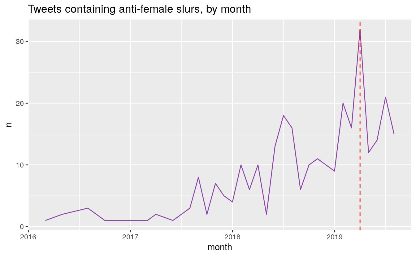
Word frequencies of slurs
Indeed, the fact the Minister McKenna is a female likely has a lot to do with the content of her replies. Let’s examine how often anti-female slurs are hurled her way.
# My code here uses an unnecessary regex string to avoid having search engines pick up the words. I am sure that readers who like puzzles will have no trouble figuring out what words I was looking at.

token_sentiment %>% filter(value == -5) %>% select(word) %>% unlist() %>%
  str_extract("(bit|sl|c|tw)(u|a|c)(t|nt|h)(es)?") %>% unique() %>%
  .[!is.na(.)] -> slurs

tweets %>% filter(str_detect(tweet, paste(slurs, collapse = "|"))) %>%
  group_by(month = as.yearmon(timestamp)) %>% count() %>%
  filter(month > "2015-11" & month < "2019-09") %>% ggplot(aes(x = month, y = n)) +
  geom_line(colour = "#8E44AD") +
  geom_vline(xintercept = as.yearmon("2019-04"), colour = "red", linetype = "dashed") +
  scale_x_continuous() +
  ggtitle("Tweets containing anti-female slurs, by month")
In late 2017, Tory MP Gerry Ritz used the “Climate Barbie” slur. He eventually apologized, but it appears to have brought the insult into the mainstream:
tweets %>% filter(str_detect(tweet, "barbie")) %>%
  group_by(month = as.yearmon(timestamp)) %>% count() %>%
  filter(month > "2015-11" & month < "2019-09") %>%
  ggplot(aes(x = month, y = n)) +
  geom_line(colour = "#F1948A") +
  geom_vline(xintercept = as.yearmon("2019-04"), colour = "red", linetype = "dashed") +
  scale_x_continuous() +
  ggtitle("Tweets containing the word \"barbie\", by month")
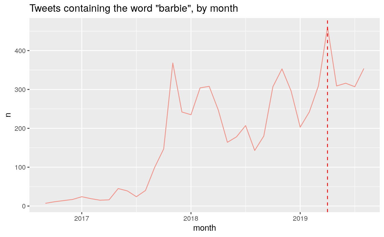
Indeed, McKenna has had to put up with many slurs in the last four years. The total counts for these slur over all replies directed to McKenna are:
censor <- function(x) {
  for (i in seq_along(x)) {
    if (x[i] == "barbie") next
    x[i] <- paste0(substr(x[i], start = 1, stop = 2),
                   paste0(rep("*", nchar(x[i]) - 3), collapse = ""),
                   substr(x[i], start = nchar(x[i]), stop = nchar(x[i])))
  }
  x
}

tweets %>%
  filter(str_detect(tweet, paste(c(slurs, "barbie"), collapse = "|"))) %>%
  mutate(slur = str_extract_all(tweet, paste(c(slurs, "barbie"), collapse = "|"))) %>%
  select(slur) %>%
  unnest(cols = c(slur)) %>%
  count(slur) %>%
  mutate(slur = censor(slur))

#> # A tibble: 5 x 2
#>   slur       n
#>   <chr>  <int>
#> 1 barbie  6961
#> 2 bi**h    158
#> 3 cu*t      32
#> 4 sl*t       6
#> 5 tw*t     107
Summary
No one should have to put up with abuse, no matter their position or their politics. I applaud Minister McKenna for her perseverance and dogged dedication to her portfolio. Since approximately the middle of 2017, she has put up with constant abuse, and yet remains accessible to Canadians via Twitter. We can see from the evidence in this post that Climate Change denial and misogyny seem to go hand-in-hand. This is definitely something I will look into more.
This post was compiled on 2020-10-09 11:36:43. Since that time, there may have been changes to the packages that were used in this post. If you can no longer use this code, please notify the author in the comments below.
Packages Used in this post
sessioninfo::package_info(dependencies = "Depends")

#>  package     * version    date       lib source
#>  assertthat    0.2.1      2019-03-21 [1] RSPM (R 4.0.0)
#>  cli           2.0.2      2020-02-28 [1] RSPM (R 4.0.0)
#>  colorspace    1.4-1      2019-03-18 [1] RSPM (R 4.0.0)
#>  crayon        1.3.4      2017-09-16 [1] RSPM (R 4.0.0)
#>  curl          4.3        2019-12-02 [1] RSPM (R 4.0.0)
#>  digest        0.6.25     2020-02-23 [1] RSPM (R 4.0.0)
#>  downlit       0.2.0      2020-09-25 [1] RSPM (R 4.0.2)
#>  dplyr       * 1.0.2      2020-08-18 [1] RSPM (R 4.0.2)
#>  ellipsis      0.3.1      2020-05-15 [1] RSPM (R 4.0.0)
#>  evaluate      0.14       2019-05-28 [1] RSPM (R 4.0.0)
#>  fansi         0.4.1      2020-01-08 [1] RSPM (R 4.0.0)
#>  farver        2.0.3      2020-01-16 [1] RSPM (R 4.0.0)
#>  fs            1.5.0      2020-07-31 [1] RSPM (R 4.0.2)
#>  generics      0.0.2      2018-11-29 [1] RSPM (R 4.0.0)
#>  ggplot2     * 3.3.2      2020-06-19 [1] RSPM (R 4.0.1)
#>  glue          1.4.2      2020-08-27 [1] RSPM (R 4.0.2)
#>  gtable        0.3.0      2019-03-25 [1] RSPM (R 4.0.0)
#>  hms           0.5.3      2020-01-08 [1] RSPM (R 4.0.0)
#>  htmltools     0.5.0      2020-06-16 [1] RSPM (R 4.0.1)
#>  htmlwidgets   1.5.1      2019-10-08 [1] RSPM (R 4.0.0)
#>  hugodown      0.0.0.9000 2020-10-08 [1] Github (r-lib/hugodown@18911fc)
#>  janeaustenr   0.1.5      2017-06-10 [1] RSPM (R 4.0.0)
#>  jsonlite    * 1.7.1      2020-09-07 [1] RSPM (R 4.0.2)
#>  knitr         1.30       2020-09-22 [1] RSPM (R 4.0.2)
#>  labeling      0.3        2014-08-23 [1] RSPM (R 4.0.0)
#>  lattice       0.20-41    2020-04-02 [1] RSPM (R 4.0.0)
#>  lifecycle     0.2.0      2020-03-06 [1] RSPM (R 4.0.0)
#>  magrittr      1.5        2014-11-22 [1] RSPM (R 4.0.0)
#>  Matrix        1.2-18     2019-11-27 [1] RSPM (R 4.0.0)
#>  munsell       0.5.0      2018-06-12 [1] RSPM (R 4.0.0)
#>  pillar        1.4.6      2020-07-10 [1] RSPM (R 4.0.2)
#>  pkgconfig     2.0.3      2019-09-22 [1] RSPM (R 4.0.0)
#>  purrr         0.3.4      2020-04-17 [1] RSPM (R 4.0.0)
#>  R6            2.4.1      2019-11-12 [1] RSPM (R 4.0.0)
#>  Rcpp          1.0.5      2020-07-06 [1] RSPM (R 4.0.2)
#>  readr       * 1.3.1      2018-12-21 [1] RSPM (R 4.0.2)
#>  rlang         0.4.7      2020-07-09 [1] RSPM (R 4.0.2)
#>  rmarkdown     2.3        2020-06-18 [1] RSPM (R 4.0.1)
#>  scales        1.1.1      2020-05-11 [1] RSPM (R 4.0.0)
#>  sessioninfo   1.1.1      2018-11-05 [1] RSPM (R 4.0.0)
#>  SnowballC     0.7.0      2020-04-01 [1] RSPM (R 4.0.0)
#>  stringi       1.5.3      2020-09-09 [1] RSPM (R 4.0.2)
#>  stringr     * 1.4.0      2019-02-10 [1] RSPM (R 4.0.0)
#>  tibble      * 3.0.3      2020-07-10 [1] RSPM (R 4.0.2)
#>  tidyr       * 1.1.2      2020-08-27 [1] RSPM (R 4.0.2)
#>  tidyselect    1.1.0      2020-05-11 [1] RSPM (R 4.0.0)
#>  tidytext    * 0.2.6      2020-09-20 [1] RSPM (R 4.0.2)
#>  tokenizers    0.2.1      2018-03-29 [1] RSPM (R 4.0.2)
#>  utf8          1.1.4      2018-05-24 [1] RSPM (R 4.0.0)
#>  vctrs         0.3.4      2020-08-29 [1] RSPM (R 4.0.2)
#>  withr         2.3.0      2020-09-22 [1] RSPM (R 4.0.2)
#>  wordcloud2  * 0.2.1      2018-01-03 [1] RSPM (R 4.0.0)
#>  xfun          0.18       2020-09-29 [2] RSPM (R 4.0.2)
#>  yaml          2.2.1      2020-02-01 [1] RSPM (R 4.0.0)
#>  zoo         * 1.8-8      2020-05-02 [1] RSPM (R 4.0.0)
#>
#> [1] /home/conor/Library
#> [2] /usr/local/lib/R/site-library
#> [3] /usr/local/lib/R/library
References
Nielsen, Finn Årup. 2011. “A New ANEW: Evaluation of a Word List for Sentiment Analysis in Microblogs.” In Proceedings of the Eswc2011 Workshop on ‘Making Sense of Microposts’: Big Things Come in Small Packages, edited by Matthew Rowe, Milan Stankovic, Aba-Sah Dadzie, and Mariann Hardey, 718:93–98. CEUR Workshop Proceedings. http://ceur-ws.org/Vol-718/paper_16.pdf.
Conor I. Anderson, PhD
Alumnus, Climate Lab
Conor is a recent PhD graduate from the Department of Physical and Environmental Sciences at the University of Toronto Scarborough (UTSC).