Examining Wintertime Polar Events at Toronto
Introduction
In my last post, I looked at December temperatures in Toronto in reponse to the cold snap that we experienced between December and January of this winter. I wanted to delve deeper and contextualize that cold snap among other prolonged periods of polar air in Toronto, which I’ll refer to as “polar events” throughout this post.
First, I will load the libraries that I will use.
library(canadaHCDx)
library(dplyr)
library(ggplot2)
library(lubridate)
library(readr)
library(reshape2)
library(tibble)
library(tidyr)
library(zoo)
We’ll get Toronto temperature data up to January 9, 2018.
# Toronto changed station code afer June 2003, so we'll merge it with the new one.
tor <- hcd_daily(5051, 1950:2003)
tmp <- hcd_daily(31688, 2003:2018)
tor <- bind_rows(tor[1:which(tor$Date == "2003-06-30"),], tmp[which(tmp$Date == "2003-07-01"):which(tmp$Date == "2018-01-09"),])
Instead of using temperature, I’m going to classify events by air masses. I’ll start with data from Sheridan’s Spatial Synoptic Classification (SSC) (Sheridan 2002).
Just like my last post, I’ll use four bins, as per Anderson and Gough ( 2017):
- ‘cool’: SSC codes 2 (dry polar) and 5 (moist polar)
- ‘moderate’: SSC codes 1 (dry moderate) and 4 (moist moderate)
- ‘warm’: SSC codes 3 (dry tropical), 6 (moist tropical), 66 (moist tropical plus), and 67 (moist tropical double plus)
- ‘transition’: SCC code 7 (transition)
I’m going to manually add some air classifications at the end of the SSC series to account for the rest of the polar event (through January 7). Those dates haven’t been officially classified under the to SSC yet. Note that I might have some of these days wrong. I used archived jet stream maps for reference.
f <- tempfile()
download.file("http://sheridan.geog.kent.edu/ssc/files/YYZ.dbdmt", f, quiet = TRUE)
air <- read_table(f, col_names = c("Station", "Date", "Air"), col_types = cols(col_character(), col_date(format = "%Y%m%d"), col_factor(levels = c(1, 2, 3, 4, 5, 6, 7, 66, 67)))) # Note, I am ignoring code 8 because that is the SSC2 "NA" value, which is turned to NA by ignoring.
levels(air$Air) <- list(cool = c(2, 5), mod = c(1, 4), warm = c(3, 6, 66, 67), trans = "7")

air <- bind_rows(air, tibble(Date = seq(ymd("2018-01-01"), ymd("2018-01-09"), by = 'day'), Air = factor(c(rep('cool', 7), 'mod', 'mod'), levels = levels(air$Air))))
Now, let’s create a table that includes just temperature and air mass data.
tor <- tor %>% select(Date, MaxTemp, MinTemp, MeanTemp) %>% add_column(Air = air$Air)
tail(tor)

#> # A tibble: 6 x 5
#>   Date       MaxTemp MinTemp MeanTemp Air
#>   <date>       <dbl>   <dbl>    <dbl> <fct>
#> 1 2018-01-04    -7.7   -19.7    -13.7 cool
#> 2 2018-01-05   -14.7   -20.6    -17.7 cool
#> 3 2018-01-06   -15.4   -22.3    -18.9 cool
#> 4 2018-01-07    -1     -17.5     -9.3 cool
#> 5 2018-01-08     3      -1.7      0.7 mod
#> 6 2018-01-09     1.6    -0.6      0.5 mod
I’m going to isolate the winter months (December, January, and February). Note that I will be using the year of January and February to refer to a given winter, so winter 2014 is December 2013 through February 2014. In the text, I will (rightfully) call this winter 2013/14.
tor_winter <- tor %>% filter(month(Date) %in% c(1, 2, 12)) %>% group_by(Year = year(Date), Month = month(Date)) %>% mutate(Winter = case_when(Month %in% c(1:11) ~ Year, Month == 12 ~ Year + 1)) %>% ungroup %>% select(-`Year`, -`Month`)
Since I’m interested in the length of polar events, I’ll look for lengths of continuous cool air using R’s
rle() function. The code below is probably overly-complicated, but it does the trick. I will count polar events as continuous periods of cool air. Days with transitional air will count if they are preceeded and followed by cool air; same goes for missing values.
fx <- function(x, y, comm = NULL, ...) {

  event <- rle(x == "cool" | (
    (is.na(x) | x == "trans") & (lag(x, 1) == "cool" & lead(x, 1) == "cool")
  ))

  event$values[event$lengths < 3] <- FALSE

  if (!inherits(comm, "function")) {
    # This will return the lengths of the polar events
    lens <- NULL
    for (i in 1:length(event[[1]])) {
      if (!is.na(event$values[i]) & event$values[i]) {
        lens <- c(lens, rep(event$lengths[i], event$lengths[i]))
      } else {
        lens <- c(lens, rep(NA, event$lengths[i]))
      }
    }
    lens
  } else {
    # This will return summary variables of the polar events
    vals <- NULL
    for (i in 1:length(event[[1]])) {
      if (!is.na(event$values[i]) & event$values[i]) {
        pull <- c(rep(FALSE, sum(event$lengths[1:(i - 1)])),
                  rep(TRUE, event$lengths[i]))
        pull <- c(pull, rep(FALSE, length(y) - length(pull)))
        vals <- c(vals, rep(comm(y[pull], ...), event$lengths[i]))
      } else {
        vals <- c(vals, rep(NA, event$lengths[i]))
      }
    }
    vals
  }
}
Using the above function, I’ll “annotate” each day that is part of a polar event with the start date, end date, and length of the cold event. I will also calculate the temperature swing as the change between each day and the previous, i.e. $t_i - t_{i-1}$.
tor_winter <- tor_winter %>%
  group_by(Winter) %>%
  mutate(Start = as.Date(fx(Air, Date, min)),
         End = as.Date(fx(Air, Date, max)),
         Length = fx(Air),
         MaxSwing = MaxTemp - lag(MaxTemp, 1),
         MinSwing = MinTemp - lag(MinTemp, 1),
         MeanSwing = MeanTemp - lag(MeanTemp, 1))
As an example, we can look at what this looks like for the recent cold snap.
tor_winter %>% filter(Start == "2017-12-21")

#> # A tibble: 18 x 12
#> # Groups:   Winter [1]
#>    Date       MaxTemp MinTemp MeanTemp Air   Winter Start      End        Length
#>    <date>       <dbl>   <dbl>    <dbl> <fct>  <dbl> <date>     <date>      <int>
#>  1 2017-12-21    -1.8    -4.7     -3.3 cool    2018 2017-12-21 2018-01-07     18
#>  2 2017-12-22    -1.8    -5.7     -3.8 cool    2018 2017-12-21 2018-01-07     18
#>  3 2017-12-23     0.6    -4.8     -2.1 cool    2018 2017-12-21 2018-01-07     18
#>  4 2017-12-24    -1.1    -4.8     -3   cool    2018 2017-12-21 2018-01-07     18
#>  5 2017-12-25    -3     -10.5     -6.8 trans   2018 2017-12-21 2018-01-07     18
#>  6 2017-12-26   -10.2   -14.4    -12.3 cool    2018 2017-12-21 2018-01-07     18
#>  7 2017-12-27    -9.9   -17.9    -13.9 cool    2018 2017-12-21 2018-01-07     18
#>  8 2017-12-28   -11.8   -19.6    -15.7 cool    2018 2017-12-21 2018-01-07     18
#>  9 2017-12-29    -7.3   -14.3    -10.8 cool    2018 2017-12-21 2018-01-07     18
#> 10 2017-12-30    -6.8   -18.1    -12.5 trans   2018 2017-12-21 2018-01-07     18
#> 11 2017-12-31   -13.7   -20.2    -17   cool    2018 2017-12-21 2018-01-07     18
#> 12 2018-01-01    -7.9   -18.6    -13.3 cool    2018 2017-12-21 2018-01-07     18
#> 13 2018-01-02    -7.1   -12.5     -9.8 cool    2018 2017-12-21 2018-01-07     18
#> 14 2018-01-03    -5.3   -11.2     -8.3 cool    2018 2017-12-21 2018-01-07     18
#> 15 2018-01-04    -7.7   -19.7    -13.7 cool    2018 2017-12-21 2018-01-07     18
#> 16 2018-01-05   -14.7   -20.6    -17.7 cool    2018 2017-12-21 2018-01-07     18
#> 17 2018-01-06   -15.4   -22.3    -18.9 cool    2018 2017-12-21 2018-01-07     18
#> 18 2018-01-07    -1     -17.5     -9.3 cool    2018 2017-12-21 2018-01-07     18
#> # … with 3 more variables: MaxSwing <dbl>, MinSwing <dbl>, MeanSwing <dbl>
I’ll wipe out any years with more than 10 missing values (i.e. 1967–1971, which are missing more than a month’s worth of data each).
tor_winter[group_indices(tor_winter) %in% which((tor_winter %>% group_by(Winter) %>% summarize(NAs = sum(is.na(Air))))$NAs > 10), 3:ncol(tor_winter)] <- NA

#> `summarise()` ungrouping output (override with `.groups` argument)
Let’s also make a traditional “seasonal” winter data set.
tor_winter_means <- tor_winter %>% group_by(Winter) %>% select(Winter, MaxTemp, MinTemp, MeanTemp) %>% summarize_all(mean, na.rm = TRUE)
Finally, we can create a summary table detailing the key characteristics of each polar event.
tor_polar_events <- tor_winter %>%
  filter(!is.na(Length)) %>%
  group_by(Winter, Start, End, Length) %>%
  summarize(ColdestDay = min(MinTemp, na.rm = TRUE),
            WarmestDay = max(MaxTemp, na.rm = TRUE),
            MaxTemp = mean(MaxTemp, na.rm = TRUE),
            MinTemp = mean(MinTemp, na.rm = TRUE),
            MeanTemp = mean(MeanTemp, na.rm = TRUE),
            MaxSwing = min(MaxSwing, na.rm = TRUE),
            MinSwing = min(MinSwing, na.rm = TRUE))

#> `summarise()` regrouping output by 'Winter', 'Start', 'End' (override with `.groups` argument)


# Let's also keep track of the proportion of air masses (especially NA)
tor_polar_events <- left_join(tor_polar_events, tor_winter %>%
                                filter(!is.na(Length)) %>%
                                group_by(Winter, Start, End, Length, Air) %>%
                                tally %>% spread(Air, n, fill = 0))

#> Joining, by = c("Winter", "Start", "End", "Length")


# Ungroup these data frames for reshaping
tor_polar_events <- ungroup(tor_polar_events)
Great! Now let’s see what we can come up with. Let’s plot the “big” events in the last 30 years. We’ll filter our data for polar events that are 10 days or longer, and that have a mean temperature below 0 °C.
gg <- melt(tor_polar_events %>% filter(Winter > 1987 , Length >= 10, MeanTemp <= 0) %>%
             mutate(Period = paste0(Start, "-", End)) %>%
             select(Period, Length, WarmestDay, ColdestDay, MaxTemp, MinTemp,
                    MeanTemp), id = c("Period", "Length"))

ggplot(gg, aes(x = Period, y = value, colour = variable, group = Period, lwd = Length)) +
  geom_line(alpha = .6) + theme(axis.text.x = element_text(size = 7, angle = 90)) +
  ylab("Temperature (°C)") + labs(colour = "Variable", lwd = "Snap Length") +
  ggtitle("\"Big\" Polar Events in Toronto since 1988")
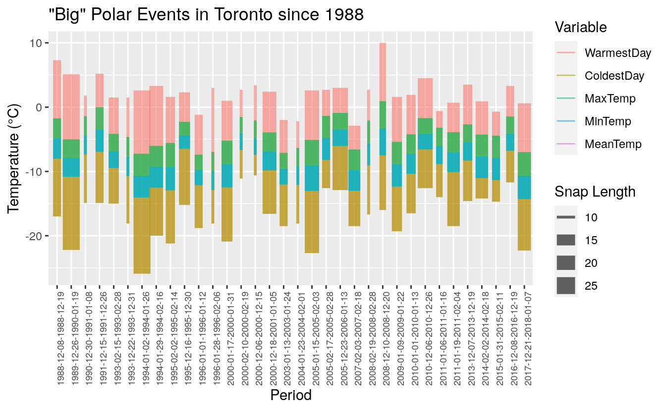
In the above graph, line width represents polar event length. The bars show the range between the extremes, and averaged $T_{max}$ and $T_{min}$; $T_{mean}$ is where the green and blue bars meet. We can already see that the December 2017 / January 2018 cold snap was among the coldest events in terms of mean temperature, and was relatively long. Let’s take a closer look and rank the polar events of the past 30 years.
last_30_cold <- filter(tor_polar_events, Winter > 1988)
last_30_tor <- filter(tor_winter_means, Winter > 1988)
These are the top 10 coldest winters (in terms of $T_{mean}$). This year is ranked 4, but we can’t take that number at face value because the series is just over one third of the length of other winters and was dominated by cold temperatures. The last few days have probably done a great deal to undo that, but any data after January 9th are omitted from this analysis!
arrange(last_30_tor, MeanTemp)

#> # A tibble: 30 x 4
#>    Winter MaxTemp MinTemp MeanTemp
#>     <dbl>   <dbl>   <dbl>    <dbl>
#>  1   1994  -2.50    -8.50    -5.51
#>  2   2014  -2.25    -8.56    -5.49
#>  3   2015  -1.83    -8.77    -5.35
#>  4   2018  -2.02    -8.50    -5.27
#>  5   1996  -0.901   -6.94    -3.93
#>  6   2011  -0.778   -7.04    -3.93
#>  7   2003  -1.05    -6.73    -3.89
#>  8   2009   0.07    -7.37    -3.66
#>  9   1990  -0.159   -6.03    -3.11
#> 10   2005   0.387   -6.54    -3.08
#> # … with 20 more rows
What about longest polar events? This recent snap was ranked 8.
arrange(last_30_cold, desc(Length))

#> # A tibble: 171 x 14
#>    Winter Start      End        Length ColdestDay WarmestDay MaxTemp MinTemp
#>     <dbl> <date>     <date>      <int>      <dbl>      <dbl>   <dbl>   <dbl>
#>  1   1990 1989-12-26 1990-01-19     25      -22.2        5.1   -5.02  -10.8
#>  2   1994 1994-01-02 1994-01-26     25      -25.9        2.6   -7.25  -14.1
#>  3   2006 2005-12-23 2006-01-13     22      -12.9        3     -0.9    -6.03
#>  4   2011 2010-12-06 2010-12-26     21      -12.6        4.5   -1.71   -6.56
#>  5   2005 2005-01-15 2005-02-03     20      -22.7        2.6   -5.10  -13.0
#>  6   1994 1994-01-29 1994-02-16     19      -20          3.3   -6.03  -12.5
#>  7   2001 2000-12-18 2001-01-05     19      -16.6        2.4   -3.93   -9.84
#>  8   2018 2017-12-21 2018-01-07     18      -22.3        0.6   -6.99  -14.3
#>  9   2011 2011-01-19 2011-02-04     17      -18.5        0.7   -3.89  -10.1
#> 10   2014 2014-02-02 2014-02-18     17      -14.2        0.9   -4.28  -11.0
#> # … with 161 more rows, and 6 more variables: MeanTemp <dbl>, MaxSwing <dbl>,
#> #   MinSwing <dbl>, cool <dbl>, trans <dbl>, `<NA>` <dbl>
How about when we look at the coldest polar event in terms of one-day temperature extremes? This year’s event was ranked 5.
arrange(last_30_cold, ColdestDay)

#> # A tibble: 171 x 14
#>    Winter Start      End        Length ColdestDay WarmestDay MaxTemp MinTemp
#>     <dbl> <date>     <date>      <int>      <dbl>      <dbl>   <dbl>   <dbl>
#>  1   1994 1994-01-02 1994-01-26     25      -25.9        2.6   -7.25   -14.1
#>  2   2015 2015-02-15 2015-02-23      9      -25.1       -2.7  -10.5    -18.1
#>  3   2016 2016-02-10 2016-02-14      5      -24.7       -0.1   -7.28   -17.6
#>  4   2005 2005-01-15 2005-02-03     20      -22.7        2.6   -5.10   -13.0
#>  5   2018 2017-12-21 2018-01-07     18      -22.3        0.6   -6.99   -14.3
#>  6   1990 1989-12-26 1990-01-19     25      -22.2        5.1   -5.02   -10.8
#>  7   2014 2014-01-07 2014-01-09      3      -22.2       -2.9   -8.8    -16.7
#>  8   2004 2004-01-05 2004-01-12      8      -22.1        0.7   -4.82   -12.1
#>  9   2004 2004-01-15 2004-01-20      6      -21.4       -2     -7.67   -15.7
#> 10   1995 1995-02-02 1995-02-14     13      -21.2        1.6   -5.57   -12.9
#> # … with 161 more rows, and 6 more variables: MeanTemp <dbl>, MaxSwing <dbl>,
#> #   MinSwing <dbl>, cool <dbl>, trans <dbl>, `<NA>` <dbl>
Which were the coldest polar events (in terms of $T_{mean}$)? The polar event this year is ranked 10.
last_30_cold %>% select(-`ColdestDay`, -`WarmestDay`) %>% arrange(MeanTemp)

#> # A tibble: 171 x 12
#>    Winter Start      End        Length MaxTemp MinTemp MeanTemp MaxSwing
#>     <dbl> <date>     <date>      <int>   <dbl>   <dbl>    <dbl>    <dbl>
#>  1   2015 2015-02-15 2015-02-23      9  -10.5    -18.1    -14.3   -13.5
#>  2   2014 2014-01-07 2014-01-09      3   -8.8    -16.7    -12.8   -18.2
#>  3   2016 2016-02-10 2016-02-14      5   -7.28   -17.6    -12.5   -10.9
#>  4   2014 2014-01-26 2014-01-29      4   -7.07   -16.4    -11.8    -7.9
#>  5   2004 2004-01-15 2004-01-20      6   -7.67   -15.7    -11.7    -5.7
#>  6   2015 2015-02-26 2015-02-28      3   -7.23   -15.8    -11.6    -1.90
#>  7   2014 2013-12-30 2014-01-02      4   -8.78   -13.2    -11.0   -12.2
#>  8   2014 2014-01-18 2014-01-23      6   -7.17   -14.7    -11.0   -12.4
#>  9   1994 1994-01-02 1994-01-26     25   -7.25   -14.1    -10.7   -11.4
#> 10   2018 2017-12-21 2018-01-07     18   -6.99   -14.3    -10.7    -7.2
#> # … with 161 more rows, and 4 more variables: MinSwing <dbl>, cool <dbl>,
#> #   trans <dbl>, `<NA>` <dbl>
Now let’s look at the largest one-day temperature change in $T_{max}$. The event this year is ranked 80.)
last_30_cold %>% select(-`ColdestDay`, -`WarmestDay`, -`MinTemp`, -`MeanTemp`) %>%
arrange(MaxSwing)

#> # A tibble: 171 x 10
#>    Winter Start      End        Length MaxTemp MaxSwing MinSwing  cool trans
#>     <dbl> <date>     <date>      <int>   <dbl>    <dbl>    <dbl> <dbl> <dbl>
#>  1   2014 2014-01-07 2014-01-09      3  -8.8      -18.2    -6.40     3     0
#>  2   1993 1993-02-06 1993-02-09      4  -4.55     -18     -20.7      3     1
#>  3   1994 1993-12-11 1993-12-13      3  -0.467    -17.3   -15.6      3     0
#>  4   1991 1991-01-21 1991-01-26      6  -5.48     -17.1   -14.5      6     0
#>  5   2000 2000-01-17 2000-01-31     15  -5.22     -16     -12.5     12     3
#>  6   2006 2006-02-18 2006-02-20      3  -4.83     -14.8    -6.7      3     0
#>  7   1996 1996-02-12 1996-02-18      7  -5.2      -14.4   -13        7     0
#>  8   1989 1989-02-02 1989-02-10      9  -4.89     -14.1    -6.1      9     0
#>  9   1995 1995-02-02 1995-02-14     13  -5.57     -13.9   -15.1     13     0
#> 10   1992 1992-01-15 1992-01-21      7  -5.94     -13.8    -5.7      7     0
#> # … with 161 more rows, and 1 more variable: `<NA>` <dbl>
Finally, we’ll look at the largest one-day temperature change in $T_{min}$. This year’s cold snap ranks 39.
last_30_cold %>% select(-`ColdestDay`, -`WarmestDay`, -`MaxTemp`, -`MeanTemp`) %>% arrange(MinSwing)

#> # A tibble: 171 x 10
#>    Winter Start      End        Length MinTemp MaxSwing MinSwing  cool trans
#>     <dbl> <date>     <date>      <int>   <dbl>    <dbl>    <dbl> <dbl> <dbl>
#>  1   1993 1993-02-06 1993-02-09      4  -13.7     -18      -20.7     3     1
#>  2   1994 1993-12-11 1993-12-13      3   -7.07    -17.3    -15.6     3     0
#>  3   1995 1995-02-02 1995-02-14     13  -12.9     -13.9    -15.1    13     0
#>  4   1991 1991-01-21 1991-01-26      6  -12.7     -17.1    -14.5     6     0
#>  5   1989 1989-02-22 1989-02-28      7   -8.5     -11.1    -14.3     6     1
#>  6   1997 1997-01-26 1997-01-31      6  -12.0      -8.1    -13.6     4     2
#>  7   1989 1989-01-01 1989-01-06      6   -9.33     -6.8    -13.6     6     0
#>  8   1991 1991-02-23 1991-02-28      6   -7.77     -7.1    -13.5     6     0
#>  9   1993 1992-12-21 1992-12-27      7   -6.26     -6.5    -13.5     6     1
#> 10   1996 1996-02-12 1996-02-18      7  -12.3     -14.4    -13       7     0
#> # … with 161 more rows, and 1 more variable: `<NA>` <dbl>
Conclusions
The cold snap this year was ranked highly in terms of length, mean temperature and coldest day, but not very highly when we consider the one-day temperature change. Indeed, it was cold, but the low temperatures arrived slowly, not suddenly. It is interesting to note that among the top polar events, we see a number in recent years. While polar events since 2000 have been cold, it seems that extreme temperature swings were more common in the 1990s. We see a handul of cold events from winter 1993/94 and the two winters that we examined in Anderson and Gough ( 2017) among the coldest and longest. I should flag that these rankings vary based on how many days of transitional air we include in the analysis, but the coldest events are relatively consistent and concentrated in the early 1990s and recent 2010s.
This post was compiled on 2020-10-09 11:13:43. Since that time, there may have been changes to the packages that were used in this post. If you can no longer use this code, please notify the author in the comments below.
Packages Used in this post
sessioninfo::package_info(dependencies = "Depends")

#>  package     * version    date       lib source
#>  assertthat    0.2.1      2019-03-21 [1] RSPM (R 4.0.0)
#>  canadaHCD   * 0.0-2      2020-10-01 [1] Github (ConorIA/canadaHCD@e2f4d2b)
#>  canadaHCDx  * 0.0.8      2020-10-01 [1] gitlab (ConorIA/canadaHCDx@0f99419)
#>  cli           2.0.2      2020-02-28 [1] RSPM (R 4.0.0)
#>  colorspace    1.4-1      2019-03-18 [1] RSPM (R 4.0.0)
#>  crayon        1.3.4      2017-09-16 [1] RSPM (R 4.0.0)
#>  curl          4.3        2019-12-02 [1] RSPM (R 4.0.0)
#>  digest        0.6.25     2020-02-23 [1] RSPM (R 4.0.0)
#>  downlit       0.2.0      2020-09-25 [1] RSPM (R 4.0.2)
#>  dplyr       * 1.0.2      2020-08-18 [1] RSPM (R 4.0.2)
#>  ellipsis      0.3.1      2020-05-15 [1] RSPM (R 4.0.0)
#>  evaluate      0.14       2019-05-28 [1] RSPM (R 4.0.0)
#>  fansi         0.4.1      2020-01-08 [1] RSPM (R 4.0.0)
#>  farver        2.0.3      2020-01-16 [1] RSPM (R 4.0.0)
#>  fs            1.5.0      2020-07-31 [1] RSPM (R 4.0.2)
#>  generics      0.0.2      2018-11-29 [1] RSPM (R 4.0.0)
#>  geosphere     1.5-10     2019-05-26 [1] RSPM (R 4.0.0)
#>  ggplot2     * 3.3.2      2020-06-19 [1] RSPM (R 4.0.1)
#>  glue          1.4.2      2020-08-27 [1] RSPM (R 4.0.2)
#>  gtable        0.3.0      2019-03-25 [1] RSPM (R 4.0.0)
#>  hms           0.5.3      2020-01-08 [1] RSPM (R 4.0.0)
#>  htmltools     0.5.0      2020-06-16 [1] RSPM (R 4.0.1)
#>  hugodown      0.0.0.9000 2020-10-08 [1] Github (r-lib/hugodown@18911fc)
#>  knitr         1.30       2020-09-22 [1] RSPM (R 4.0.2)
#>  labeling      0.3        2014-08-23 [1] RSPM (R 4.0.0)
#>  lattice       0.20-41    2020-04-02 [1] RSPM (R 4.0.0)
#>  lifecycle     0.2.0      2020-03-06 [1] RSPM (R 4.0.0)
#>  lubridate   * 1.7.9      2020-06-08 [1] RSPM (R 4.0.2)
#>  magrittr      1.5        2014-11-22 [1] RSPM (R 4.0.0)
#>  munsell       0.5.0      2018-06-12 [1] RSPM (R 4.0.0)
#>  pillar        1.4.6      2020-07-10 [1] RSPM (R 4.0.2)
#>  pkgconfig     2.0.3      2019-09-22 [1] RSPM (R 4.0.0)
#>  plyr          1.8.6      2020-03-03 [1] RSPM (R 4.0.2)
#>  purrr         0.3.4      2020-04-17 [1] RSPM (R 4.0.0)
#>  R6            2.4.1      2019-11-12 [1] RSPM (R 4.0.0)
#>  rappdirs      0.3.1      2016-03-28 [1] RSPM (R 4.0.0)
#>  Rcpp          1.0.5      2020-07-06 [1] RSPM (R 4.0.2)
#>  readr       * 1.3.1      2018-12-21 [1] RSPM (R 4.0.2)
#>  reshape2    * 1.4.4      2020-04-09 [1] RSPM (R 4.0.2)
#>  rlang         0.4.7      2020-07-09 [1] RSPM (R 4.0.2)
#>  rmarkdown     2.3        2020-06-18 [1] RSPM (R 4.0.1)
#>  scales        1.1.1      2020-05-11 [1] RSPM (R 4.0.0)
#>  sessioninfo   1.1.1      2018-11-05 [1] RSPM (R 4.0.0)
#>  sp            1.4-2      2020-05-20 [1] RSPM (R 4.0.0)
#>  storr         1.2.1      2018-10-18 [1] RSPM (R 4.0.0)
#>  stringi       1.5.3      2020-09-09 [1] RSPM (R 4.0.2)
#>  stringr       1.4.0      2019-02-10 [1] RSPM (R 4.0.0)
#>  tibble      * 3.0.3      2020-07-10 [1] RSPM (R 4.0.2)
#>  tidyr       * 1.1.2      2020-08-27 [1] RSPM (R 4.0.2)
#>  tidyselect    1.1.0      2020-05-11 [1] RSPM (R 4.0.0)
#>  utf8          1.1.4      2018-05-24 [1] RSPM (R 4.0.0)
#>  vctrs         0.3.4      2020-08-29 [1] RSPM (R 4.0.2)
#>  withr         2.3.0      2020-09-22 [1] RSPM (R 4.0.2)
#>  xfun          0.18       2020-09-29 [2] RSPM (R 4.0.2)
#>  yaml          2.2.1      2020-02-01 [1] RSPM (R 4.0.0)
#>  zoo         * 1.8-8      2020-05-02 [1] RSPM (R 4.0.0)
#>
#> [1] /home/conor/Library
#> [2] /usr/local/lib/R/site-library
#> [3] /usr/local/lib/R/library
References
Anderson, Conor I., and William A. Gough. 2017. “Evolution of Winter Temperature in Toronto, Ontario, Canada: A Case Study of Winters 2013/14 and 2014/15.” Journal of Climate 30 (14): 5361–76. https://doi.org/10.1175/JCLI-D-16-0562.1.
Sheridan, Scott C. 2002. “The Redevelopment of a Weather-Type Classification Scheme for North America.” International Journal of Climatology 22 (1): 51–68. https://doi.org/10.1002/joc.709.
Conor I. Anderson, PhD
Alumnus, Climate Lab
Conor is a recent PhD graduate from the Department of Physical and Environmental Sciences at the University of Toronto Scarborough (UTSC).